Journal of Machine Intelligence and Data Science (JMIDS)

1. Introduction

In the realm of chemical engineering, the core of processes often resides in their reactions. Certain reactions have garnered heightened focus owing to their practicality, significance, and economic viability. Among these pivotal reactions within chemical processes lies the catalytic conversion of sulfur dioxide (SO₂) to sulfur trioxide (SO₃). The conversion of SO₂ has two domains of applications: the mitigation of pollution and the production of sulfuric acid (H₂SO₄). This reaction is based on the following stoichiometric equilibrium expressed by Equation (1):

(1)

For the first application, it is uncontested that urban population growth has sparked an industrial activity boom that has significantly increased the amount of air contaminants such as SO₂ [1]–[3]. To remove SO₂ emanating from coal-fired power plants and mitigate pollution, industries use a variety of flue gas desulfurization (FGD) methods. FGD processes are essential for reducing air pollution caused by sulfur dioxide emissions. FGD processes can broadly be classified into two main categories: wet processes and dry processes [4]–[7]. Wet processes, the most used technologies, involve the utilization of limestone or slaked lime slurry as sorbents in spray towers, enabling chemical absorption to eliminate SO₂. Wet processes can eliminate up to 99% of the pollutant, producing a significant amount of hazardous material. On the other hand, dry processes involve the physical or chemical sorption of SO₂ on materials such as activated carbon or other sorbents, typically implemented in a fixed bed configuration [8]–[10]. Through the various technologies to remove SO₂, some also rely on its oxidation [8]–[12].

For the latter application, the SO₂ oxidation is the most important step in manufacturing H₂SO₄, the most-produced chemical product worldwide [13]–[15]. It is used in several applications such as the manufacturing of phosphate fertilizers and a variety of other chemicals. It plays a role in metal processing, it serves as an electrolyte in lead-acid car batteries, and it is employed in the petroleum refining industry to remove impurities from fuel as well as other refinery products [16]–[18]. Using a catalyst bed, SO₂ is oxidized to produce SO₃ (Equation (1)). The oxidation of SO₂ is an exothermic reversible reaction, influenced by temperature and pressure, and is typically performed industrially in an adiabatic packed bed reactor [19]–[21]. At temperatures exceeding 400°C, the reverse reaction becomes progressively favored, leading to a decrease in the achievable conversion of SO₂ as the temperature increases. However, it is worth noting that there is a minimum operating temperature of common SO₂ oxidation catalysts, often referred to as the strike temperature, which is also around 400°C. Balancing these conflicting requirements is achieved through the implementation of multistage catalytic reactors and inter-stage cooling. In the following process step, slightly diluted H₂SO₄ (usually as 97-98% H₂SO₄ containing 2-3% water) and SO₃ are reacted to produce more concentrated H₂SO₄, as given by Equation (2) [22], [23].

(2)

The conversion of SO₂ to SO₃ relies heavily on the catalyst performance. While vanadium, platinum, and iron-based catalysts have been the primary focus of numerous studies, other metals have also been considered [24]–[27]. According to the available literature, catalysts such as sodium-vanadium, platinum-palladium, platinum, and platinum-tin are widely recognized for their predominant use in FGD. These catalysts have demonstrated their effectiveness in facilitating the desired chemical reactions involved in the removal of SO₂ from flue gases [1], [28], [29]. The rate of SO₂ conversion can be significantly influenced by the combination of different metals in varying quantities, particularly in promoted or bimetallic catalysts. For instance, research has demonstrated that SO₂ oxidation promoters like alkaline-earth metals, namely potassium, sodium, and cesium, strengthen the structure and bonding of the catalyst. As a result, vanadium oxide based catalysts with promoters exhibit improved conversion [30]–[32]. Therefore, in the context of H₂SO₄ production, commonly employed catalysts include potassium-vanadium, cesium-vanadium, platinum, and mixtures containing vanadium combined with other compounds and/or promoters such as calcium, copper, iron, barium, manganese, and magnesium [33]–[35]. Ongoing research and development efforts aim to explore new catalyst formulations and modifications, enhancing their efficiency and durability in both applications.

The selection and optimization of catalysts play a critical role in ensuring effective SO₂ oxidation for sulfur removal and H₂SO₄ production [30]. However, due to a large number of parameters in any catalytic reaction including catalyst properties and operating variables, establishing analytical correlations between all these variables and the resultant steady-state conversion is challenging. Furthermore, the proliferation of diverse catalyst types encompassing a wide array of compositions exacerbates the difficulty in identifying the most optimal catalyst type and composition. In addressing this challenge, the integration of machine learning (ML) models is promising in elucidating the underlying nonlinear relationships between variables and in the pursuit of optimal operating conditions, and aids in selecting the most suitable catalyst type and composition.

Numerous researchers have employed diverse experimental catalytic strategies, varying in operating parameters such as temperature, pressure, and concentrations of inlet feed gases [27], [36], [37]. Nevertheless, there is frequently a paucity of comprehensive information regarding the optimal catalyst(s) and their corresponding compositions for the desired operating conditions [30]. Consequently, robust methodologies for handling nonlinear relationships and optimization techniques have garnered recent attention. ML methodologies, such as artificial neural networks (ANNs), present a promising avenue for constructing nonlinear models incorporating all relevant variables to ascertain the optimal catalyst and its composition, thereby enhancing both efficiency and conversion. Despite the growing utilization of ML methodologies across various disciplines, its application within the catalysis domain remains nascent [38]. The major reason is the lack of universal datasets in catalytic activities [39]. Catalyst development often relies on empirical trial-and-error methods based on physio-chemical properties, necessitating significant time and effort to identify optimal solutions. Automated ML approaches have demonstrated efficacy in refining models, elucidating catalytic mechanisms, and generating innovative concepts for catalytic design [38]–[43].

This study relies on a comprehensive dataset on the catalytic conversion of SO₂ [30], updated to 2023, with a diverse array of catalysts and operating parameters. The dataset, which includes two ranges of SO₂ mole fractions (below 1% for FGD and above 7% for H₂SO₄ production), is refined for accuracy and consistency. An optimal ANN model is identified through meticulous hyperparameter tuning (to optimize the ANN model's architecture and parameters) and used within a multi-objective optimization (MOO) framework to address trade-offs in the conversion process and generate the Pareto domain. The study uses the non-dominated sorting genetic algorithm (NSGA-II) and the net flow method (NFM) to identify and rank Pareto-optimal solutions. This approach integrates advanced computational methodologies with chemical engineering principles, contributing to efficiency enhancement and cost reduction in catalytic processes.

2. Methods

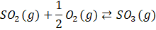
This study comprises three primary sections. The initial section focuses on the development of an ANN model. Within this section, data collection is conducted, followed by rigorous preprocessing techniques to ensure data integrity. Hyperparameter tuning is subsequently employed to optimize the ANN's performance, involving the construction and evaluation of multiple ANN models. The final model selection is based on the comparative performance assessment of each model. The second section entails the formulation of three distinct objectives, which are framed as a MOO problem. Utilizing the NSGA-II, the Pareto domain – a set of solutions representing the trade-offs between conflicting objectives – is identified. In the third and final section, a multi-criteria decision-making approach known as NFM is applied to rank the solutions approximating the Pareto domain. This method facilitates the identification of the optimal solution. The procedural workflow is illustrated in Figure 1.

Each section of this study will be explained in detail, providing comprehensive coverage of the respective steps involved. Furthermore, the rationale behind each methodological choice will be discussed, along with its relevance and contribution to the overall research objectives.

2. 1. Artificial Neural Network Model Development

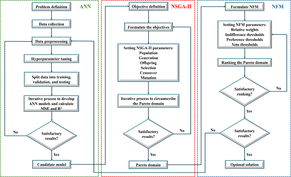
In 1943, McCulloch and Pitts proposed a computational model inspired by the human brain, which sparked research on ANNs [44]. ANN models have the ability to learn, recognize, and solve complex problems. Among the several types of ANNs, feedforward neural networks (FFNNs) are particularly interesting due to their structural representation as a computational model in a network form. This structural representation is what allows FFNNs to be a universal function approximator, capable of approximating any continuous function [45]. The FFNN can address a broad range of problems related to pattern recognition and prediction. This ability has been embraced by various researchers, who have appreciated FFNNs for their universal approximation ability [45]–[47]. FFNNs are computational models that comprise multiple interconnected neurons or nodes, arranged in a layered structure, where each layer is connected in a forward direction to the preceding layer. These neural networks have a specific structural configuration (Figure 2a) and are capable of processing information through the synaptic links or weights that connect the nodes (Figure 2b).

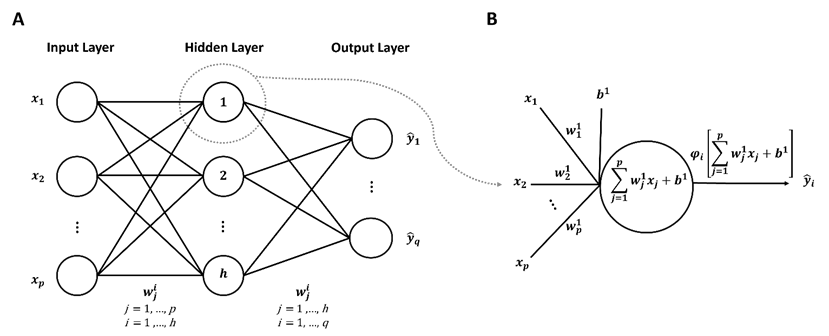
The process of supervised learning involves minimizing a cost function expressed as the difference between the desired output y_i and the output of the model . Various cost functions can be defined for this purpose. For example, mean squared error (MSE) is a commonly used cost function in regression problems, which can be expressed as [45]:

(3)

where N is the number of training points and q is the number of output neurons.

There are various conventional derivative-based methods, such as Quasi-Newton [48], Levenberg-Marquardt [49], adaptive moment estimation (Adam) [50], etc. used to adjust the connection weights to minimize the cost function. Adam is a popular algorithm for solving complex issues involving a large number of variables or data.

As depicted in Figure 1, the initial step in the implementation of an ANN involves defining the problem statement. In the context of this project, the objective is to construct an ANN model capable of predicting the conversion of SO₂. Following the problem definition, the subsequent step entails the acquisition of raw data. While direct experimentation within a specific system necessitates considerable resources in terms of time, labor, infrastructure, and financial investment, a more practical approach involves leveraging existing literature, which encompasses a wealth of research findings accessible online. Across various domains of chemical engineering, extensive experimental data have been amassed over numerous decades. However, collating this data is a labor-intensive endeavor, requiring a meticulous review of potential sources to ascertain their relevance to the project and extract pertinent information.

The inclusion criteria of data from scientific articles within the dataset necessitate the documentation of catalytic activity tests employing heterogeneous catalysts. Furthermore, these articles must provide details regarding the experimental conditions, encompassing independent variables, as well as the outcomes of these tests, represented by dependent variables. The dataset thus encompasses a spectrum of information including the composition and properties of the catalysts (e.g., specific surface area, pore characteristics, particle size), synthesis methodologies (e.g., calcination parameters such as temperature and time), operating conditions including temperature, pressure, catalyst mass, inlet volumetric flowrate, as well as the mole fractions of O₂ and SO₂ within the system. Additionally, the dataset incorporates the conversion of SO₂ as the system's output variable.

For the dataset preparation, a comprehensive screening process was undertaken, considering 152 literature papers, culminating in the identification of 32 papers deemed suitable for data extraction. Numerous considerations influenced the selection criteria for inputs into the final database. Notably, a significant challenge arose from the inconsistent reporting of information within some of the candidate papers, resulting in the omission of certain variables. Consequently, catalysts and promoters characterized by a paucity of data points and minimal variance were excluded from consideration as final inputs.

Table 1 presents the finalized list of the input and output variables within the database. Notably, 14 active metals and promoters emerged as the preferred candidates for inclusion, along with three support materials denoted by binary indicators reflecting their presence or absence. Furthermore, operating parameters such as temperature, pressure, the ratio of catalyst weight to volumetric flow rate (W/V), and the mole fractions of SO₂ and O₂ complete the list of input variables. The output variable, representing the conversion of SO₂ to SO₃, completes the database structure. Although additional variables such as pore volume, pore size, and surface area were gathered from the literature review, they were not included in the main dataset due to the substantial amounts of data not reported in many papers.

Table 1. SO₂ conversion databank description with 22 input variables and one output variable used to develop the ANN model to predict conversion.

ANN Variables	Description	Unit	Mean	Standard deviation	Min	Max
Calcium	Active metal / promoter	Mass fraction (%)	0.088	0.386	0	2.257
Ceria		Mass fraction (%)	0.123	0.662	0	4.885
Cesium		Mass fraction (%)	1.183	2.936	0	11.05
Copper		Mass fraction (%)	0.012	0.003	0	0.024
Iron		Mass fraction (%)	0.044	0.189	0	1.832
Lanthanum		Mass fraction (%)	0.094	0.687	0	6.826
Magnesium		Mass fraction (%)	0.001	0.010	0	0.100
Manganese		Mass fraction (%)	0.019	0.118	0	0.750
Palladium		Mass fraction (%)	0.022	0.144	0	2
Platinum		Mass fraction (%)	0.539	1.497	0	9.091
Potassium		Mass fraction (%)	4.052	5.545	0	18.428
Sodium		Mass fraction (%)	0.034	0.384	0	5.463
Tin		Mass fraction (%)	0.153	0.473	0	2.200
Vanadium		Mass fraction (%)	1.904	2.059	0	8
Alumina	Support material	0 or 1	0.161	0.367	0	1
Titania		0 or 1	0.065	0.246	0	1
Silicate		0 or 1	0.775	0.418	0	1
Temperature	Operating parameter	°C	457	90	204	799
Pressure		Atm	1.535	1.864	1	10
W/V		kgcat·s/L	4.223	8.819	0.003	28.379
SO2		Mole fraction (%)	6.022	4.358	0.001	20
O2		Mole fraction (%)	13.292	5.299	0.03	20.393
SO2 Conversion	Output	%	61.187	30.978	0	100

Following the data collection, the subsequent stage entails preprocessing to render the raw data suitable for their utilization within a ML algorithm. Data preprocessing serves to facilitate the management and manipulation of complex datasets, a task that often necessitates a considerable amount of processing time [51]. Despite its pivotal role in model development, data preprocessing is occasionally overlooked compared to other stages; nevertheless, it typically consumes over 50% of the total time allocated to data mining endeavors [52]. Various techniques are employed in the preprocessing phase to enhance the quality of datasets, and these techniques will be succinctly discussed in the subsequent discussion.

Data in real-world scenarios often contains incompleteness, noise, and inconsistency. Consequently, data-cleaning efforts aim to address these issues meticulously by identifying outliers and rectifying inconsistencies within the dataset [53]. In this study, outliers were identified and removed from the dataset. Acknowledging the equal significance of all data elements, data normalization emerges as an essential data transformation technique employed to standardize all data elements within a predefined range [54]. This normalization process not only expedites the learning phase within neural network backpropagation algorithms but also mitigates the potential dominance of attributes with larger ranges and/or values over attributes with smaller ranges and/or values [55]. In this work, min/max normalization was used to transfer the data to a range between 0 and 1. Furthermore, data transformation may serve as an effective strategy for reducing the dimensionality of input data, particularly when correlations exist among a series of variables. Principal component analysis (PCA) stands out as a widely adopted method in this regard [56]. Therefore, the use of PCA for data reduction was explored. In the current case study, given the low level of correlation among the input variables and especially for the large number of independent catalysts, the PCA did not result in a smaller number of input variables and was not found useful.

ML models generally assume datasets are complete, but missing values are often encountered during data collection [51], [57]. To manage this, various data preprocessing techniques, including methods like autoassociative neural networks (AANNs), are employed for imputing missing data [58]. In this work, some missing data included pore size, pore volume, surface area, calcination time, temperature, and preparation methods. However, the effectiveness of AANNs is influenced by the correlation between variables [59]. In this case study, the AANN model struggled to accurately predict missing values due to the low correlation among features. As a result, the variables with missing values were removed from the main dataset, despite their recognized importance.

It is important to stress that to reach the final model, the procedure depicted in Figure 1 is not achieved in a single pass, but rather through multiple iterations. In this investigation, the main effort was devoted to the management and validation of the databank, especially determining which data points from the literature would be useful for inclusion in the databank. Initially, all literature data containing the necessary information were considered. However, some catalysts had a very limited number of instances and were removed from the database. Other papers had instances with identical inputs but with different conversions due to disparities in catalyst properties. In this case, the average conversion was calculated for similar data points, and this single average value was used to replace the redundant data points in the database.

According to Figure 1, the subsequent step following preprocessing entails in conducting hyperparameter tuning to identify the optimal parameters for the ANN model. Enhancing the model's performance and minimizing errors necessitate the careful selection of the neural network's structure and associated parameters [60]. While the number of neurons in the input and output layers remains fixed to correspond with the model's inputs and outputs, respectively, the configuration of intermediate layers (hidden layers), as well as the number of neurons within each hidden layer, the number of epochs, the batch size, the learning rate, the optimizer, and the activation functions must be specified. These parameters play a pivotal role and can significantly influence model performance. Initially, models are constructed with parameters based on prior knowledge and expertise, with the initial weights assigned as small random values. In case of overfitting or underfitting, hyperparameter tuning techniques are employed to identify optimal parameters, aiming to minimize MSE for the validation set. These techniques often leverage grid search, random search, Bayesian optimization, and many other methodologies [60], [61]. Ultimately, the selection of the final model involves a trade-off between model simplicity and MSE value, striking a balance to achieve satisfactory performance [60].

During the hyperparameter tuning phase, a series of models were trained using the 5-fold cross-validation and random search method to optimize parameters across two distinct ANN architectures. The first architecture consisted of three hidden layers while the second had five hidden layers. Throughout this process, certain parameters were held constant, namely a sigmoid as the activation function, a learning rate of 0.01, 2000 epochs, and a batch size of 32. The following parameters were varied: the number of layers, the number of neurons within each layer, and the optimizer methods (Adam or Nadam). Numerous models were subsequently trained, with variations introduced by altering the fixed parameters.

As depicted in Figure 1, the subsequent procedural step is to partition the data records into three distinct subsets: the training set, the validation set, and the testing set. Different combinations were randomly tested, and the best combination was selected for the best model. In the subsequent phase depicted in Figure 1, the effectiveness of the constructed ANN model is assessed utilizing various criteria. Performance metrics serve to evaluate the goodness of the fit of the ML regression models [62]. The most common performance metrics are the root mean squared error (RMSE), mean absolute error (MAE), MSE, Pearson correlation coefficient, and coefficient of determination (R²). In this study, MSE and R² are used.

2.2. Multi-Objective Optimization

In the field of engineering, ML is typically used in synergy with an optimization algorithm to determine the set of process input variables that optimizes specific objective functions to operate chemical processes under optimal conditions [63]–[66]. MOO problems are optimization problems that must satisfy multiple, often conflicting, objectives [28]. A solution is defined as a vector of decision variables X= {x₁,x₂,x₃,…,x_n } that optimizes the vector of objective functions F(X)= {f₁ (X),f₂ (X), f₃(X),…,f_M (X)} within a feasible region of solutions which may be subjected to equality h_g (X) and inequality g_h (X) constraints. The decision variables are bounded between lower (x_min) and upper (x_max) limits, which constrain the search space for each variable [67]–[69]. This process is mathematically represented by Equation (4).

(4)

where M is the number of objectives. Each of the objective functions where M is the number of objectives. Each of the objective functions f_m(X) can be either minimised or maximised [70]. A maximization problem can be converted into a minimization by negating the objective function [71]. With conflicting objectives, improving one objective may worsen the other objectives. The concept of Pareto optimality can address this issue [71], [72] using the dominance relationship in an unbiased way to generate a large number of Pareto-optimal solutions rather than a single aggregate optimal solution. These solutions are referred to as non-dominated solutions. It is then up to a decision maker to select the best one among all Pareto-optimal solutions based on his/her preferences [67]. can be either minimised or maximised [70]. A maximization problem can be converted into a minimization by negating the objective function [71]. With conflicting objectives, improving one objective may worsen the other objectives. The concept of Pareto optimality can address this issue [71], [72] using the dominance relationship in an unbiased way to generate a large number of Pareto-optimal solutions rather than a single aggregate optimal solution. These solutions are referred to as non-dominated solutions. It is then up to a decision maker to select the best one among all Pareto-optimal solutions based on his/her preferences [67].

MOO techniques aim to identify a diverse set of solutions that reside on the Pareto front. These techniques, particularly the evolutionary MOO algorithms, are designed to circumscribe as accurately as possible the Pareto domain while overcoming challenges such as infeasible regions, local optima, and smooth regions of objective functions. Balancing computational cost and efficiency is crucial in addressing these challenges [73], [74]. Various methods are available for solving MOO problems, with multi-objective evolutionary algorithms (MOEAs) being a popular choice [72]–[77]. MOEAs utilize the dominance relationships in their quest to uncover Pareto-optimal solutions, a strategy shared by other optimization methods [78]. While MOEAs are effective in finding global optima and demonstrating robustness against noise, they have limitations, including potential redundancy and significant computational time [79].

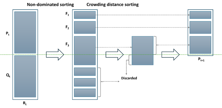
NSGA-II is a popular method within MOEAs. It is specially designed to tackle MOO problems and identify Pareto-optimal solutions. NSGA-II operates on the principles of elitism, an explicit diversity mechanism, and prioritization of non-dominated solutions. At each generation (t), the parent population (P_t) undergoes standard genetic operations such as selection, crossover, and mutation to generate the offspring population (Q_t). These two populations are then merged to form a new population (R_t) comprising 2N individuals. R_t is segmented into various non-dominance groups, and the new population of N fittest individuals is populated sequentially with points from the front with the least number of the domination score to fronts with higher domination scores. The selection of points in the last front necessary to reach N individuals is made in such a way as to maximize diversity in the population of solutions using the crowding distance criterion. Figure 3 provides a visual representation of the process used at each generation [71].

In various chemical engineering applications, particularly in processes like SO₂ oxidation, the development of ML models presents an opportunity to optimize complex systems by leveraging optimization algorithms. In this work, the optimization framework aims at maximizing conversion and productivity while minimizing catalyst cost, to strike a balance between these competing objectives.

The conversion (X) of SO₂, defined in Equation (5), is calculated from the ANN model.

(5)

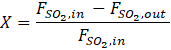
where F_SO2,in and F_SO2 are the input and output molar flowrates of SO₂, respectively. The productivity is defined as the rate at which the moles of SO₂ are converted to SO₃ per unit time and per unit mass of the catalyst expressed by Equation (6).

(6)

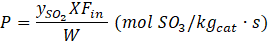
where y_SO2 is the input SO₂ mole fraction, F_in is the total inlet molar flowrate, and W is the catalyst weight. This equation can be transformed in terms of the catalyst weight to the volumetric flow rate ratio under standard conditions (1 atm, 0^oC) as well as expressing y_SO2 and X in percentage as per Table 1 and the input to the AAN model (Equation (7)).

(7)

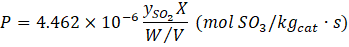
where W/V is the ratio of the weight of the catalyst bed and the volumetric flow rate in kg_cat·s/L. The third objective function is the cumulative cost of catalysts used in the process. This objective function involves a linear relationship between the mass fractions of individual catalysts and their corresponding costs (Equation (8)).

(8)

where r is the number of catalysts in the databank, c_i is the price of each catalyst and m_i is the mass fraction of each catalyst. The list of prices of the catalysts has been obtained using the Bloomberg databank and it is reported in Table 2 [80], [81].

Table 2. Estimated price of each catalyst.

S.N.	Catalyst	Symbol	Price ($/kg)
1	Calcium	Ca	5
2	Cerium	Ce	4
3	Cesium	Cs	13000
4	Copper	Cu	8
5	Iron	Fe	0.5
6	Lanthanum	La	4
7	Magnesium	Mg	3.5
8	Manganese	Mn	2
9	Palladium	Pd	43500
10	Platinum	Pt	32000
11	Potassium	K	850
12	Sodium	Na	300
13	Tin	Sn	30
14	Vanadium	V	250

2. 3. Multi-Criteria Decision Making

Once the Pareto domain is established based on domination principles (as depicted in Figure 1), the subsequent step involves ranking all non-dominated solutions. This ranking process requires the input of the decision-maker's preferences, which guide the selection of solutions according to the chosen ranking method. In this study, the NFM, a multi-criteria decision-making technique, is employed for ranking all Pareto-optimal solutions. The NFM incorporates the decision-maker's preferences through the utilization of four factors, which are outlined below [15].

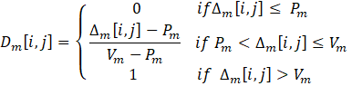
The first factor involves assigning relative weights (W_m) to each criterion or objective 'm', indicating their importance. The sum of all relative weights must be equal to one. The second factor, known as the indifference threshold (Q_m), defines the difference in the values of objective 'm' between two solutions for which it is inconclusive to favor one solution over another for that specific objective. The third factor, the preference threshold (P_m), represents the threshold beyond which the difference in objective 'm' values between two solutions warrants a preference for the solution with the better objective value. Lastly, the veto threshold (V_m) is used to rule out the selection of one solution over another if the difference between their objective 'm' values exceeds a certain threshold. The latter implies that even if a solution excels in other criteria, it may be disregarded based on a specific objective. The three thresholds are established individually for each criterion, in such a manner that:

(9)

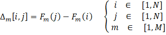
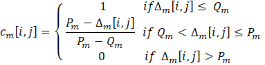
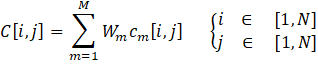
Equations (10-13) are used to calculate the various indices: the difference ∆_m[i,j] between the objective m of solutions i and j, the individual concordance index c_m[i,j], the global concordance index c[i,j], and the discordance index D_m[i,j] . These indices are determined through a pairwise comparison. When the difference between values is less than the indifference threshold for a given criterion, the individual concordance index is assigned a value of unity. Within the range spanning from the indifference to the preference thresholds, the index diminishes linearly from 1 to 0. If the difference surpasses the preference threshold for a given criterion, the concordance index is set to zero. When the difference between values is below the preference threshold, the discordance index is assigned a value of 0. Within the range encompassing the preference and veto thresholds, the index exhibits a linear progression from 0 to 1. In instances where the difference exceeds the veto threshold, the discordance index is fixed at a value of 1.

(10)

(11)

(12)

(13)

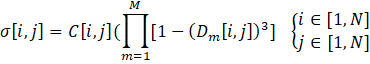
Once the global concordance and discordance indices have been calculated, the process moves on to the comparative analysis of each pair of Pareto-optimal solutions. This evaluation involves calculating each element of the outranking matrix, denoted as σ[i,j] using Equation (14). Essentially, the outranking matrix serves as a tool to determine which solutions outperform others based on their relative performance.

(14)

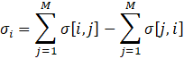
In order to determine the best solution, the score of each solution i is calculated using Equation (15). The first term assesses how well solution i performs compared to all the other solutions in the Pareto domain. The second term evaluates the performance of all the other solutions relative to solution i. After computing the ranking score for each solution, they are sorted in descending order. This calculation is the final step in the solution evaluation process. The solution with the highest score is considered the best.

(15)

3. Results and discussion

3.1. Final ANN Model

As previously explained, various ANN models were trained and integrated into the MOO phase to circumscribe the Pareto domain and propose the optimal solution for catalytic SO₂ conversion. Initially, data were gathered from diverse sources, and a subset of variables was selected. The first version of our database was formed by extracting data from 32 papers. Then, the preprocessing stage was performed to increase the integrity and quality of the data. After finalizing the input and output parameters, several ANN model structures were randomly selected to assess their ability to predict conversion. Simultaneously exploring the structure of ANNs, the hyperparameters tuning was performed to enhance the performance of the ANNs and reduce errors. This procedure is guided by experience in developing ANNs, but still involves a degree of trial and error. Once the best-performing ANN model was identified, it was used in the MOO procedure, along with the solution ranking algorithm as per Figure 1, to determine the optimal solution.

Multiple ANN models were trained using the updated hyperparameters obtained from the hyperparameter tuning process. The architecture of the final ANN model, as detailed in Table 3, consists of three hidden layers, each accommodating 22 neurons. The model employs the Adam optimizer with a learning rate set at 0.0005. Additionally, a batch size of 32 and an epoch value of 50000 were selected. The dataset was partitioned into the training, validation, and testing sets in an 80:10:10 ratio, denoted as Tr/V/Te.

Table 3. Structure of the final ANN model.

Optimizer	Learning rate	Hidden layers with neurons	Batch size	Epoch	Tr/V/Te size
Adam	0.0005	3 HL: 22, 22, 22	32	36782	80/10/10

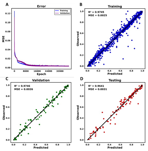
Figure 4 provides an overview of the performance of the final ANN model. As shown in Figure 4a, the MSE in the prediction of the normalized conversion for both the training and validation datasets decreases sharply at the beginning and then gradually converges to its final value as the number of epochs exceeds 10000, with the final weights and biases being recorded at 36782 epochs which were achieved with early stopping technique which can help improve the generalization performance of a model.. The parity plot of the conversion for the training data is displayed in Figure 4b, which shows an MSE of 0.0025 and an R² value of 0.9745. Figure 4c and Figure 4d further illustrate the performance of the ANN model on the validation and testing datasets, respectively. The model’s performance on these datasets is comparable to that of the training data, indicating its consistency. This uniformity across different datasets implies that the model exhibits a low error in the prediction of the conversion and can effectively generalize to unseen testing data, thereby mitigating any concerns regarding overfitting.

To comprehensively assess the capacity of the ANN model to surpass conventional statistical and regression techniques, its performance was benchmarked against linear regression, ridge regression, and polynomial regression models on a 10% testing dataset. The comparative results, presented in Table 4, highlight the superior performance of the ANN model in all evaluated metrics. Notably, the ANN model exhibits a marked improvement over its counterparts, as evidenced by significantly lower MSE and higher R² values. This analysis underscores the ANN model's robust predictive capability, achieving both greater accuracy and better generalizability compared to the tested regression approaches.

The dataset, as mentioned earlier, comprises information about two specific applications of SO₂ catalytic conversion: FGD and H₂SO₄ production. Both processes convert SO₂ into SO₃ using different metal catalysts supported by various materials. A key distinguishing factor between these applications within the dataset is the mole fraction of SO₂ in the feed. Data points with a low SO₂ concentration (less than 1%) correspond to FGD, whereas those with a higher concentration (above 7%) are associated with H₂SO₄ production.

This study primarily focuses on optimizing the production of H₂SO₄, given its significant economic importance as one of the most widely produced chemicals worldwide. However, exploring optimal conditions for FGD applications is also achievable since the data points in the dataset are comprised of both applications. Consequently, to tailor the problem formulation specifically for H₂SO₄ production, the mole fraction of SO₂ was fixed at 10%. Additionally, to mimic industrial practice, the oxygen concentration was set at 11%.

Table 4. Comparative performance of the final ANN and traditional regression models on the testing data.

Performance criteria	Linear regression	Ridge regression	Polynomial regression	ANN
MSE	0.0461	0.0463	0.0128	0.0031
R2	0.4970	0.4939	0.8597	0.9641

3. 2. Case study 1: Vanadium-potassium catalyst

The MOO problem allows for the exploration of various combinations of metals, either individually or in conjunction, supported by the three available support materials. However, given the impracticality of examining all possible combinations, a prominent bimetallic catalyst featuring a mixture of vanadium and potassium was first selected for further investigation in the MOO problem. This selection was motivated by the prevalence of reported instances involving these two metals, which collectively constitute approximately 35% of the entire databank.

Table 5 presents the fixed and variable parameters that have been set for the MOO problem. The fraction of the active phase was selected to be optimized along with operating parameters such as temperature, pressure, and the W/V. It is important to note that each variable was constrained within its range of gathered data in the databank as reported in Table 1. The temperature range was set between 310-622°C, which is the range where both vanadium and potassium coexist. The pressure was kept constant at 1 atm, while the W/V was allowed to vary between 0.02-1.00 kg_cat·s/L. The lower limit of 0.02 for W/V corresponds to the smallest W/V ratio observed when both vanadium and potassium are present in the dataset. The support material was also specified to be silica, as this material is the only one in the dataset that was used for both vanadium and potassium-based catalysts.

Table 5. Values of the decision parameters for the catalytic combination of vanadium and potassium.

Decision Parameters	State	Value
Components	Fixed	V and K
Active phase fraction	Variable	V = 2.0-8.0 wt% K = 2.0-18.42 wt%
Support	Fixed	SiO2
Temperature	Variable	310-622°C
Pressure	Fixed	1 atm
Catalyst W/V	Variable	0.02-1.00 kgcat·s/L
SO2 fraction	Fixed	0.10
O2 fraction	Fixed	0.11

Process variables that were not involved in this specific case study were set to zero. The size of the population and the number of generations of NSGA-II were respectively set at 1000 and 10000. Other NSGA-II factors depicted in Figure 1 were carefully adjusted to circumscribe a well-defined Pareto front. The selection of these parameters guides the optimization process within the MOO framework, facilitating the exploration of diverse solutions while ensuring robustness and efficiency in identifying non-dominated solutions.

The next phase involved the ranking of all Pareto-optimal solutions by the NFM, as shown in Figure 1. Table 6 outlines the set of parameters of the NFM used in this study to rank all solutions of the Pareto domain. The relative weights for the conversion and productivity were set at 0.45, whereas the weight for the cost was set at 0.1. A higher significance was placed on the first two objectives. This strategic emphasis underscores the objective of having both high conversion and high productivity, albeit potentially resulting in higher costs. Furthermore, in the NFM ranking algorithm, the specification of the indifference, preference, and veto thresholds often involves some form of expert judgment or statistical analysis. The selection of these thresholds is a critical aspect of the NFM ranking algorithm, as they directly influence the resulting ranking of all Pareto-optimal solutions.

Table 6. NFM parameters for vanadium and potassium case study.

Parameters	Conversion	Productivity	Cost
W	0.45	0.45	0.1
Q	2	0.01	50
P	5	0.03	100
V	10	0.1	200

Figure 5 provides a visual representation of the Pareto domain, highlighting the interaction among the three objective functions. In Figure 5, the three-dimensional Pareto domain is represented by three two-dimensional projections. All Pareto-optimal solutions are partitioned based on their ranking using different colors as per the legend of Figure 5b. Figure 5a examines the relationship between conversion and productivity. Conversion is defined as the extent to which SO₂ is transformed into SO₃ during the catalytic process, while productivity quantifies the speed to achieve this conversion. A preliminary analysis of the Pareto domain reveals two distinct phenomena. Firstly, both conversion and productivity generally increase simultaneously. Second, a clear conflict among these objectives is also revealed when examining the ranking partitions, where a trade-off situation is observed with the enhancement of conversion, which inevitably leads to a decrease in productivity. This inverse correlation is more visually apparent at the right edge of the Pareto domain with the highest conversion percentages coinciding with the lowest productivity values. The highest-ranked solution, namely the champion, is located at the highest productivity accompanied of a relatively small compromise in the conversion percentage.

Figure 5b explores the relationship between the percentage conversion and the cost of the catalyst of Pareto-optimal solutions. The NFM relative weight for the cost was 0.1 compared to 0.45 for the other two objectives as they were seen as more significant. It is therefore not surprising to find the highest-ranked solution at a higher cost, which implies a larger amount of catalyst to favor higher conversion and productivity. The plot of Figure 5b clearly show the conflict that exists between the desire to maximize conversion and minimize the cost. Figure 5c further investigates the relationship between cost and productivity. Concentrating on the right edge of the Pareto domain, it is clear that minimizing the cost results in lower productivity. Considering the three objectives and the relative weight for each, the champion solution was located at the highest productivity (0.193 mol SO₃/kg_cat·s), relatively high conversion (86.3%), and a high cost (163.3$/kg), resulting from the greater priority attributed to the conversion and productivity.

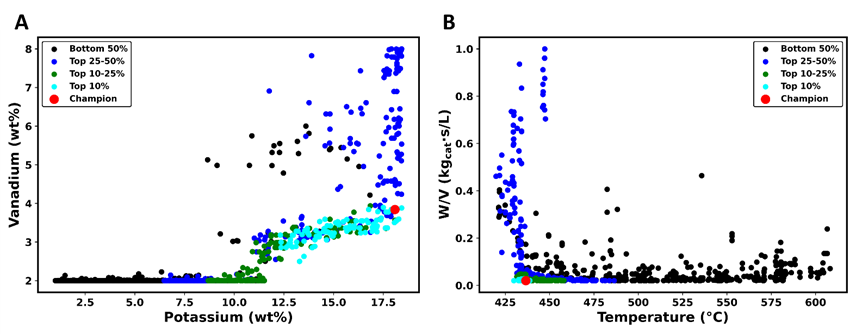
Our attention is now turned to the decision space. In this case, the composition of the selected catalyst, W/V, and the reaction temperature were the process variables that were allowed to vary. Figure 6 presents the plots of the four decision variables associated with all Pareto-optimal solutions. Figure 6a presents a plot depicting the active phase fraction for vanadium and potassium. Higher amounts of these metals are associated with increased percentage conversion, productivity, and cost. The region containing the highly-ranked Pareto-optimal solutions is located at a high fraction of potassium (17%) and a fraction of vanadium between 3 and 4%. For lower fractions of potassium, the fraction of vanadium is located at its lower value. The best Pareto-optimal solution corresponds to vanadium and potassium mass fractions of 3.8% and 18%, respectively.

Figure 6b provides an overview of the other two decision variables: the W/V ratio and the temperature. Near the strike temperature, in the vicinity of 400-425^oC, there is a sharp increase in the W/V ratio when decreasing temperature which implies a larger amount of catalyst is required to achieve higher conversion and productivity. In addition, the rate of reaction is lower at a lower temperature. Above this limiting temperature, the W/V ratio hovers around its bounded lower limit. It is important to recall that the SO₂ to SO₃ reaction is a reversible exothermic reaction such that increasing the temperature eventually leads to a decrease in the achievable conversion and productivity. It is therefore not surprising to observe the highly-ranked Pareto-optimal solutions are located in a very narrow range of temperatures just slightly above the strike temperature. The champion is obtained with a W/V value of 0.02 kg_cat·s/L and a temperature of 436°C, consistent with the reported strike temperature for the SO₂ reaction. This finding underscores the critical balance required between the amount of catalyst and the reaction temperature needed to maximize conversion and productivity, while also minimizing the negative impact of the temperature increase on the reaction equilibrium concentration.

3. 3. Case study 2: Platinum catalyst

An additional case study was undertaken to investigate the catalyst platinum and determine the optimal active phase and operating conditions. The selection of platinum for this investigation is motivated by two main factors. Firstly, platinum is renowned for its potent active sites and its high catalytic efficiency [82], [83]. Secondly, platinum-related data constitutes approximately 20% of the information gathered in the databank. Akin to the preceding case study, the objective was to determine the optimal composition and operating parameters for platinum supported on silica, under a fixed pressure of 1 atm, and fixed mole fractions of SO₂ and O₂ at 10% and 11% respectively. Therefore, the variables under consideration are the active phase fraction of platinum, temperature, and W/V.

The same ANN model employed in optimizing other metals was also applied to platinum, given that it was trained on all available metals. During the MOO phase, the lower and upper bounds of the decision variables were set based on the minimum and maximum values observed for each variable when the platinum active phase was non-zero. This approach ensures that the extrapolation does not exceed the dataset's range for each specific metal. The remaining parameters of NSGA-II were kept consistent with the previous case study. However, the NFM parameters for this case study needed to be adjusted due to differing objective ranges compared to vanadium and potassium. This adjustment was necessary because of the platinum's wider operating range and considerably higher cost compared to vanadium and potassium. Table 7 outlines the NFM parameters used in the platinum case study. Notably, the emphasis is placed on conversion and productivity over cost, as depicted in Table 7.

Table 7. NFM parameters for platinum case study.

Parameters	Conversion	Productivity	Cost
W	0.45	0.45	0.1
Q	1	0.2	300
P	5	0.4	700
V	10	1.0	1500

Figure 7 presents the Pareto domain for the platinum case study, focusing on the same three objectives previously considered: conversion, productivity, and catalyst cost. In Figure 7a, a consistent pattern emerges, akin to the vanadium-potassium case study, where two similar trends are observed. Examining the oblique left edge of the Pareto domain, it is clear that higher conversion is accompanied by higher productivity to a certain point. This trend makes sense as the definition of productivity embeds the conversion. However, examining the colored bands of similarly-ranked Pareto-optimal solutions and the right edge of the Pareto domain shows a clear trend of the decrease in productivity as the conversion continues to increase. This trend is logical since to achieve very high conversion, the flowing gas must spend significantly more time in the reactor and/or a greater amount of platinum catalyst must be used. As a result, the productivity decreases as it includes both the reaction time and the amount of catalyst. Indeed, it is possible to achieve near 100% conversion, but at the expense of reduced productivity. Additionally, Figure 7b corroborates the notion that increased conversion demands a larger amount of the catalyst's active phase, consequently increasing the overall cost. Figure 7c elucidates the interplay between cost and productivity. Notably, it reveals that achieving high productivity does not inherently entail incurring exorbitant costs. This suggests that high productivity levels can be attained without substantial increases in cost, particularly when the amount of platinum used is minimal. This highlights the feasibility of optimizing productivity while mitigating costs. The highest-ranked Pareto-optimal solution is achieved at a percentage conversion of 90%, a productivity of 1.34 mol SO₃/kg_cat·s, and a cost of $294/kg. It is important to recognize that this result does not simulate the steady-state process involved in H₂SO₄ production, where the goal is to achieve nearly 100% conversion. This high conversion is attained using multiple packed beds with intermediate heat exchangers, where the temperature and conversion vary continuously along the packed bed. The results of the current investigation are for a constant temperature and steady-state homogeneous process.

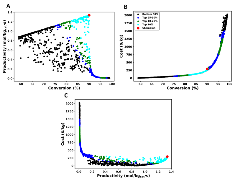
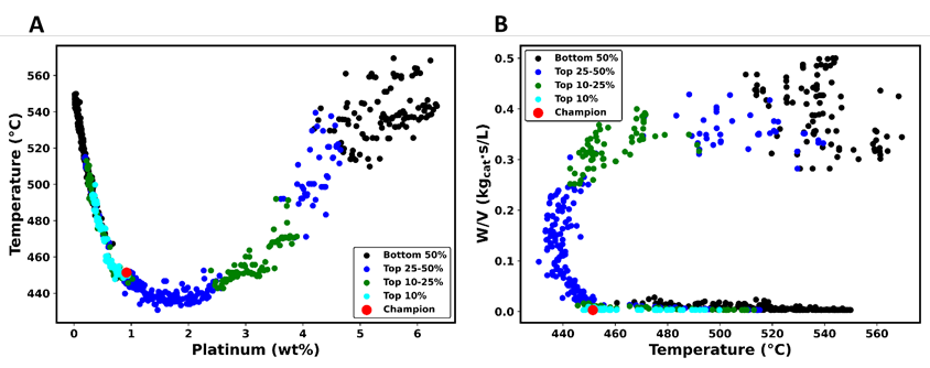
Figure 8 depicts the decision space corresponding to the Pareto domain illustrated in Figure 7. This analysis offers valuable insights into the relationship between temperature, the platinum active phase, and W/V ratio. In Figure 8a, the temperature variation is juxtaposed with changes in the platinum active phase. Initially, temperature bounds were set within the range of 204-780°C. However, the MOO process has identified Pareto-optimal solutions in a temperature range spanning 430-570°C. Figure 8a can be partitioned into three distinct sections based on the platinum active phase concentration.

The first portion of the plot of Figure 8a encompasses instances where the platinum concentration remains below 1%. Within this range, increasing the platinum active phase content coincides with enhanced conversion and productivity, particularly at lower temperatures. Remarkably, this region aligns with the lower segment of Figure 8b representing the W/V ratio. This juxtaposition indicates that within this zone, optimal productivity levels alongside a 90% conversion are attainable when the temperature is on the low side. In the second segment of Figure 8a, the temperature remains relatively constant as the platinum active phase concentration increases. This phenomenon is mirrored in Figure 8b, where at low and nearly constant temperature, the W/V ratio exhibits an upward trend. Consequently, this trend corresponds to an increasing percentage conversion, and at the same time, there is a trade-off in terms of reduced productivity.

The third segment of Figure 8a illustrates a simultaneous increase in the temperature and the amount of platinum active phase. This trend is also evident in Figure 8b, particularly at higher values of the W/V ratio. With an increase in the amount of the platinum active phase, in the temperature, and the W/V ratio, the productivity decreases while the percentage conversion and the catalyst cost surge to peak levels. A delicate balance between conversion efficiency and overall productivity must be managed. While achieving peak percentage conversion, care must be exercised to mitigate costs.

The methodologies developed in this study offer significant real-world applications across various industries, facilitating optimized catalyst design and operating conditions for enhanced efficiency, cost-effectiveness, and sustainability. In the H₂SO₄ production industry, this approach can be used to improve conversion and productivity while simultaneously minimizing costs and resource consumption. By applying the optimization techniques, designers can precisely tailor catalyst compositions and reaction conditions, thereby achieving higher yields and reduced energy requirements. Similarly, in the field of FDG, the method can be utilized to meet stringent environmental regulations by optimizing catalysts for SO₂ removal, ensuring both cost-efficiency and compliance with environmental standards. In the petrochemical sector, the framework can enhance the refinement of various products, increasing the selectivity and yield of desired compounds while lowering production costs. In hydrogen production, the same optimization process can balance energy consumption and catalyst performance, extending the lifespan of catalysts while maintaining high efficiency. Moreover, the methods are applicable to emerging sustainable technologies, such as carbon capture and utilization, and biomass conversion, where optimizing catalysts can significantly improve reaction outcomes and reduce waste. By integrating ANN predictions with MOO, industries can accelerate the design and testing of catalysts, reducing the need for costly and time-consuming experimental work. This integrated approach not only drives innovation but also provides a pathway to solving complex challenges in a range of sectors, from chemical production to energy generation. Overall, the insights gained from this study can be leveraged to foster sustainable, efficient, and cost-effective operations, benefiting industries seeking to improve both their economic outcomes and environmental performance.

4. Conclusion

The catalytic conversion of SO₂ is critical in various industrial applications, including FGD and H₂SO₄ production. This study delves into optimizing this conversion process using a multifaceted approach that incorporates ML, MOO, and decision-making techniques. Our efforts shed light on the complex interplay between various parameters and objectives, providing valuable insights into enhancing conversion efficiency while balancing productivity and cost considerations, even for a relatively simple reactive system. In this study, data were gathered from literature sources and underwent preprocessing to improve their quality. The hyperparameter tuning was then conducted to identify the best AAN model to predict SO₂ conversion with the lowest error. Using this AAN model, three objectives (conversion, productivity, and cost of the catalyst) were formulated, and the NSGA-II optimization algorithm was used to circumscribe the Pareto domain. The Pareto-optimal solutions were subsequently ranked using the NFM.

Two case studies were considered for H₂SO₄ production: one using a vanadium-potassium catalyst and the other using platinum as the catalyst. For each case study, the same AAN model obtained to predict conversion was utilized, and along with other objectives, the Pareto domain and optimal decision variables were illustrated. It was observed that for both case studies, conversion and productivity have trade-offs; increasing one objective leads to a decrease in the other. These trade-offs also impact the cost of the catalysts. The analysis underscored the critical role of key parameters, such as catalyst composition, temperature, and W/V ratio, in shaping process performance. Optimal solutions often required careful adjustments to these parameters, reflecting the delicate balance needed to achieve desired conversion levels without compromising productivity or incurring excessive costs. The optimal findings for the first case study revealed a conversion of 86.3%, a productivity of 0.193 mol SO₃/kg_cat·s, and a cost of 163.3$/kg with vanadium and potassium mass fractions of 3.8% and 18%, respectively. These outcomes were acheived with an optimal W/V value of 0.02 kg_cat·s/L and a temperature of 436°C. For the second case study, a conversion of 90%, a productivity of 1.34 mol SO₃/kg_cat·s, and a cost of $294/kg were obtained. These results were achieved with 1% platinum wt% and with a W/V value of 0.003 kg_cat·s/L and a temperature of 451°C.

In conclusion, this study offers a comprehensive exploration of the catalytic conversion of SO₂, integrating ML, MOO, and decision-making techniques to optimize process performance. By leveraging advanced methodologies and rigorous analysis, we elucidated key insights into the intricate dynamics governing conversion efficiency, productivity, and cost. Our findings pave the way for informed decision-making and strategic optimization initiatives aimed at enhancing the sustainability and efficiency of catalytic conversion processes in diverse industrial sectors.

Acknowledgement

The authors acknowledge the Natural Sciences and Engineering Research Council of Canada (NSERC) for funding this research. We also express our gratitude to the Digital Research Alliance of Canada for providing the platform to run the Python programs.

References

[1] A. Islam, S. H. Teo, C. H. Ng, Y. H. Taufiq-Yap, S. Y. T. Choong, and M. R. Awual, “Progress in recent sustainable materials for greenhouse gas (NOx and SOx) emission mitigation,” Progress in Materials Science, vol. 132, art. 101033, 2022.
[2] E. A. Lowe and L. K. Evans, “Industrial ecology and industrial ecosystems,” Journal of cleaner production, vol. 3, no. 1–2, pp. 47–53, 1995.
[3] M. Z. Jacobson, Air pollution and global warming: history, science, and solutions. 2nd ed., Cambridge University Press, 2012.
[4] R. K. Srivastava, W. Jozewicz, and C. Singer, “SO2 scrubbing technologies: a review,” Environmental Progress, vol. 20, no. 4, pp. 219–228, 2001.
[5] T. U. Gound, V. Ramachandran, and S. Kulkarni, “Various methods to reduce SO2 emission-a review,” International Journal of Ethics in Engineering & Management Education, vol. 1, no. 1, pp. 1–6, 2014.
[6] M. A. Hanif, N. Ibrahim, and A. Abdul Jalil, “Sulfur dioxide removal: An overview of regenerative flue gas desulfurization and factors affecting desulfurization capacity and sorbent regeneration,” Environmental Science and Pollution Research, vol. 27, no. 22, pp. 27515–27540, 2020.
[7] M. M. X. Lum, K. H. Ng, S. Y. Lai, A. R. Mohamed, A.G. Alsultan, Y. H. Taufiq-Yap, M. K. Koh, M. A. Mohamed, D. -V. N. Vo, M. Subramaniam, K. S. Mulya, and N. , Imanuella, “Sulfur dioxide catalytic reduction for environmental sustainability and circular economy: A review,” Process Safety and Environmental Protection, vol. 176, pp. 580–604, 2023.
[8] N. Karatepe, “A comparison of flue gas desulfurization processes,” Energy Sources, vol. 22, no. 3, pp. 197–206, 2000.
[9] K. H. Ng, S. Y. Lai, N. F. M. Jamaludin, and A. R. Mohamed, “A review on dry-based and wet-based catalytic sulphur dioxide (SO2) reduction technologies,” Journal of Hazardous Materials, vol. 423, art. 127061, 2022.
[10] R. del Valle-Zermeño, J. Formosa, and J. M. Chimenos, “Wet flue gas desulfurization using alkaline agents,” Reviews in Chemical Engineering, vol. 31, no. 4, pp. 303–327, 2015.
[11] R. Duan W. Chen, Z. Chen, J. Gu, Z. Dong, B. He, L. Liu, and X. Wang, “Mechanistic and Experimental Study of the CuxO@C Nanocomposite Derived from Cu3(BTC)2 for SO2 Removal,” Catalysts, vol. 12, no. 7, art. 689, 2022.
[12] R. Chen, T. Zhang, Y. Guo, J. Wang, J. Wei, and Q. Yu, “Recent advances in simultaneous removal of SO2 and NOx from exhaust gases: Removal process, mechanism and kinetics,” Chemical Engineering Journal, vol. 420, art. 127588, 2021.
[13] W. G. Davenport, M. J. King, B. Rogers, and A. Weissenberger, “Sulphuric acid manufacture,” Southern African Pyrometallurgy, Johannesburg, 2006, vol. 1, pp. 1–16.
[14] S. Sidana, “Sulfuric acid production using catalytic oxidation,” international journal of engineering and technical research, vol. 6, pp. 65–68, 2016.
[15] M. R. Zaker, C. Fauteux-Lefebvre, and J. Thibault, “Modelling and Multi-Objective Optimization of the Sulphur Dioxide Oxidation Process,” Processes, vol. 9, no. 6, art. 1072, 2021.
[16] F. García-Labiano, F. Diego, L. F. de, A. Cabello, P. Gayán, A. Abad, J. Adánez, and G. Sprachmann, “Sulphuric acid production via Chemical Looping Combustion of elemental sulphur,” Applied Energy, vol. 178, pp. 736–745, 2016.
[17] N. Vangapally, T. R. Penki, Y. Elias, S. Muduli, S. Maddukuri, S. Luski, D. Aurbach, and S. K. Martha, “Lead-acid batteries and lead–carbon hybrid systems: A review,” Journal of Power Sources, vol. 579, art. 233312, 2023.
[18] G. Kutney, Sulfur: history, technology, applications and industry, Toronto: ChemTec Publishing, 2023.
[19] W. Moeller and K. Winkler, “The double contact process for sulfuric acid production,” Journal of the Air Pollution Control Association, vol. 18, no. 5, pp. 324–325, 1968.
[20] A. A. Kiss, C. S. Bildea, and J. Grievink, “Dynamic modeling and process optimization of an industrial sulfuric acid plant,” Chemical Engineering Journal, vol. 158, no. 2, pp. 241–249, 2010.
[21] A. O. Oni, D. A. Fadare, S. Sharma, and G. P. Rangaiah, “Multi-objective optimisation of a double contact double absorption sulphuric acid plant for cleaner operation,” Journal of Cleaner Production, vol. 181, pp. 652–662, 2018.
[22] N. G. Ashar and K. R. Golwalkar, A practical guide to the manufacture of sulfuric acid, oleums, and sulfonating agents, Switzerland: Springer International Publishing, 2013.
[23] M. Tejeda-Iglesias, J. Szuba, R. Koniuch, and L. Ricardez-Sandoval, “Optimization and modeling of an industrial-scale sulfuric acid plant under uncertainty,” Industrial & Engineering Chemistry Research, vol. 57, no. 24, pp. 8253–8266, 2018.
[24] J. Loskyll, K. Stöwe, and W. F. Maier, “Search for New Catalysts for the Oxidation of SO2,” ACS Combinatorial Science, vol. 15, no. 9, pp. 464–474, 2013.
[25] X. Wang, A. Wang, N. Li, X. Wang, Z. Liu, and T. Zhang, “Catalytic reduction of SO2 with CO over supported iron catalysts,” Industrial & engineering chemistry research, vol. 45, no. 13, pp. 4582–4588, 2006.
[26] M. S. Wilburn and W. S. Epling, “Formation and decomposition of sulfite and sulfate species on Pt/Pd catalysts: An SO2 oxidation and sulfur exposure study,” ACS Catalysis, vol. 9, no. 1, pp. 640–648, 2018.
[27] X. Du, J. Xue, X. Wang, Y. Chen, J. Ran, and L. Zhang, “Oxidation of sulfur dioxide over V2O5/TiO2 catalyst with low vanadium loading: A theoretical study,” The Journal of Physical Chemistry C, vol. 122, no. 8, pp. 4517–4523, 2018.
[28] A. Shokri, F. Rabiee, and K. Mahanpoor, “Employing a novel nanocatalyst (Mn/Iranian hematite) for oxidation of SO2 pollutant in aqueous environment,” International Journal of Environmental Science and Technology, vol. 14, pp. 2485–2494, 2017.
[29] P. Yuan, H. Ma, B. Shen, and Z. Ji, “Abatement of NO/SO2/Hg0 from flue gas by advanced oxidation processes (AOPs): Tech-category, status quo and prospects,” Science of The Total Environment, vol. 806, art. 150958, 2022.
[30] A. Boucheikhchoukh, J. Thibault, and C. Fauteux‐Lefebvre, “Catalyst design using artificial intelligence: SO2 to SO3 case study,” The Canadian Journal of Chemical Engineering vol. 98, no. 9, pp. 2016–2031, 2020.
[31] X. Wang, Y. Kang, J. Li, and D. Li, “Influence of cerium and cesium promoters on vanadium catalyst for sulfur dioxide oxidation,” Korean Journal of Chemical Engineering, vol. 36, pp. 650–659, 2019.
[32] M. Mazidi, R. M. Behbahani, and A. Fazeli, “Ce promoted V2O5 catalyst in oxidation of SO2 reaction,” Applied Catalysis B: Environmental, vol. 209, pp. 190–202, 2017.
[33] F. J. Doering and D. A. Berkel, “Comparison of kinetic data for KV and CsV sulfuric acid catalysts,” Journal of Catalysis, vol. 103, no. 1, pp. 126–139, 1987.
[34] A. Nikiforova, O. Kozhura, and O. Pasenko, “Leaching of vanadium by sulfur dioxide from spent catalysts for sulfuric acid production,” Hydrometallurgy, vol. 164, pp. 31–37, 2016.
[35] L. G. Simonova, Y. O. Bulgakova, O. B. Lapina, and B. S. Bal’zhinimaev, “Catalytic properties of alkali-promoted vanadium catalysts for oxidation of sulfur dioxide,” Kinetics and catalysis, vol. 38, no. 6, pp. 820–824, 1997.
[36] T. Wang, J. Liu, Y. Yang, Z. Sui, Y. Zhang, J. Wang, and W. -P. Pan, “Catalytic conversion of mercury over Ce doped Mn/SAPO-34 catalyst: Sulphur tolerance and SO2/SO3 conversion,” Journal of hazardous materials, vol. 381, art. 120986, 2020.
[37] M. Mazidi, R. Mosayebi Behbahani, and A. Fazeli, “Screening of treated diatomaceous earth to apply as V2O5 catalyst support,” Materials Research Innovations, vol. 21, no. 5, pp. 269–278, 2017.
[38] B. R. Goldsmith, J. Esterhuizen, J.-X. Liu, C. J. Bartel, and C. Sutton, “Machine learning for heterogeneous catalyst design and discovery,” American Institute of Chemical Engineers, vol. 64, no. 7, pp. 2311–2323, 2018.
[39] T. Toyao, Z. Maeno, S. Takakusagi, T. Kamachi, I. Takigawa, and K. Shimizu, “Machine Learning for Catalysis Informatics: Recent Applications and Prospects,” Acs Catalysis, vol. 10, no. 3, pp. 2260–2297, 2020.
[40] H. Xin, “Catalyst design with machine learning,” Nature Energy, vol. 7, no. 9, pp. 790–791, 2022.
[41] T. Kurogi, M. Etou, R. Hamada, and S. Sakai, “Catalyst Design by Machine Learning and Multiobjective Optimization,” Journal of the Japan Petroleum Institute, vol. 64, no. 5, pp. 256–260, 2021.
[42] Y. Guan, D. Chaffart, G. Liu, Z. Tan, D. Zhang, Y. Wang, J. Li, and L. Ricardez-Sandoval, “Machine learning in solid heterogeneous catalysis: Recent developments, challenges and perspectives,” Chemical Engineering Science, vol. 248, art. 117224, 2022.
[43] P. Schlexer Lamoureux, K. T. Winther, J. A. Garrido Torres, V. Streibel, M. Zhao, M. Bajdich, F. Abild‐Pedersen, and T. Bligaard, “Machine learning for computational heterogeneous catalysis,” ChemCatChem, vol. 11, no. 16, pp. 3581–3601, 2019.
[44] W. S. McCulloch and W. Pitts, “A logical calculus of the ideas immanent in nervous activity,” The Bulletin of Mathematical Biophysics, vol. 5, pp. 115–133, 1943.
[45] V. K. Ojha, A. Abraham, and V. Snášel, “Metaheuristic design of feedforward neural networks: A review of two decades of research,” Engineering Applications of Artificial Intelligence, vol. 60, pp. 97–116, 2017.
[46] K. Hornik, M. Stinchcombe, and H. White, “Multilayer feedforward networks are universal approximators,” Neural networks, vol. 2, no. 5, pp. 359–366, 1989.
[47] G.-B. Huang, L. Chen, and C. K. Siew, “Universal approximation using incremental constructive feedforward networks with random hidden nodes,” IEEE Transactions on Neural Networks, vol. 17, no. 4, pp. 879–892, 2006.
[48] P. E. Gill and W. Murray, “Quasi-Newton methods for unconstrained optimization,” MA Journal of Applied Mathematics, vol. 9, no. 1, pp. 91–108, 1972.
[49] D. W. Marquardt, “An algorithm for least-squares estimation of nonlinear parameters,” Journal of the Society for Industrial and Applied Mathematics, vol. 11, no. 2, pp. 431–441, 1963.
[50] D. P. Kingma and J. Ba, “Adam: A method for stochastic optimization,” ArXiv Prepr. ArXiv14126980, 2014.
[51] S. García, S. Ramírez-Gallego, J. Luengo, J. M. Benítez, and F. Herrera, “Big data preprocessing: methods and prospects,” Big Data Analytics, vol. 1, no. 1, pp. 1–22, 2016.
[52] H. S. Obaid, S. A. Dheyab, and S. S. Sabry, “The impact of data pre-processing techniques and dimensionality reduction on the accuracy of machine learning,” in 9th annual information technology, electromechanical engineering and microelectronics conference (iemecon), IEEE, 2019, pp. 279–283.
[53] X. Chu, I. F. Ilyas, S. Krishnan, and J. Wang, “Data cleaning: Overview and emerging challenges,” in Proceedings of the international conference on management of data, San Francisco Ca, 2016, pp. 2201–2206.
[54] D. Singh and B. Singh, “Investigating the impact of data normalization on classification performance,” Applied Soft Computing, vol. 97, art. 105524, 2020.
[55] J. S. Malik, P. Goyal, and A. K. Sharma, “A comprehensive approach towards data preprocessing techniques & association rules,” in Proceedings of the 4th National Conference, vol. 132, 2010.
[56] H. Abdi and L. J. Williams, “Principal component analysis,” Wiley Interdisciplinary Reviews: Computational Statistics, vol. 2, no. 4, pp. 433–459, 2010.
[57] H. Wang and S. Wang, “Mining incomplete survey data through classification,” Knowledge and Information Systems, vol. 24, pp. 221–233, 2010.
[58] M. A. Kramer, “Autoassociative neural networks,” Computers & Chemical Engineering, vol. 16, no. 4, pp. 313–328, 1992.
[59] F. Agin, J. Thibault, and C. Fauteux‐Lefebvre, “Autoassociative neural network for missing data imputation: A case study via the styrene production process,” The Canadian Journal of Chemical Engineering, vol. 103, no. 1, pp. 339–358.
[60] T. Yu and H. Zhu, “Hyper-parameter optimization: A review of algorithms and applications,” ArXiv Prepr. ArXiv200305689, 2020.
[61] M. Feurer and F. Hutter, “Hyperparameter optimization,” Automated Machine Learning: Methods, Systems, Challenges, pp. 3–33, 2019.
[62] J. G. D. Gooijer and R. J. Hyndman, “25 years of time series forecasting,” International Journal of Forecasting, vol. 22, no. 3, pp. 443–473, 2006.
[63] Q. Qu, Z. Ma, A. Clausen, and B. N. Jørgensen, “A comprehensive review of machine learning in multi-objective optimization,” in 4th International Conference on Big Data and Artificial Intelligence (BDAI), IEEE, 2021, pp. 7–14.
[64] M. Safari, A. Sohani, and H. Sayyaadi, “A higher performance optimum design for a tri-generation system by taking the advantage of water-energy nexus,” Journal of Cleaner Production, vol. 284, art. 124704, 2021.
[65] G. P. Rangaiah and A. Bonilla-Petriciolet, Multi-objective optimization in chemical engineering: developments and applications. John Wiley & Sons, 2013.
[66] G. P. Rangaiah, Z. Feng, and A. F. Hoadley, “Multi-objective optimization applications in chemical process engineering: Tutorial and review,” Processes, vol. 8, no. 5, art. 508, 2020.
[67] J. L. J. Pereira, G. A. Oliver, M. B. Francisco, S. S. Cunha, and G. F. Gomes, “A review of multi-objective optimization: methods and algorithms in mechanical engineering problems,” Archives of Computational Methods in Engineering, vol. 29, no. 4, pp. 2285–2308, 2022.
[68] G. Chiandussi, M. Codegone, S. Ferrero, and F. E. Varesio, “Comparison of multi-objective optimization methodologies for engineering applications,” Computers & Mathematics with Applications, vol. 63, no. 5, pp. 912–942, 2012.
[69] C. Baril, S. Yacout, and B. Clément, “Design for Six Sigma through collaborative multiobjective optimization,” Computers & Industrial Engineering, vol. 60, no. 1, pp. 43–55, 2011.
[70] M. Ojha, K. P. Singh, P. Chakraborty, and S. Verma, “A review of multi-objective optimisation and decision making using evolutionary algorithms,” International Journal of Bio-Inspired Computation, vol. 14, no. 2, pp. 69–84, 2019.
[71] K. Deb, Multi-objective optimisation using evolutionary algorithms: an introduction. Springer, 2011.
[72] K. Miettinen, Nonlinear multiobjective optimization,. Springer Science & Business Media, vol. 12, 1999.
[73] K. Deb, “Introduction to evolutionary multiobjective optimization,” In Multiobjective optimization: Interactive and evolutionary approaches, Berlin, 2008, pp. 59–96.
[74] G. F. Gomes, F. A. de Almeida, P. da Silva Lopes Alexandrino, S. S. da Cunha, B. S. de Sousa, and A. C. Ancelotti, “A multiobjective sensor placement optimization for SHM systems considering Fisher information matrix and mode shape interpolation,” Engineering with Computers., vol. 35, pp. 519–535, 2019.
[75] M. Zeleny, “Compromise programming,” Multiple Criteria Decision Making, University of South Carolina Press, Columbia, pp. 262-301, 1973.
[76] N. Gunantara, “A review of multi-objective optimization: Methods and its applications,” Cogent Engineering, vol. 5, no. 1, art. 1502242, 2018.
[77] G. O. Odu and O. E. Charles-Owaba, “Review of multi-criteria optimization methods–theory and applications,” IOSR Journal of Engineering, vol. 3, no. 10, pp. 01–14, 2013.
[78] L. T. Bui and S. Alam, Multi-objective optimization in computational intelligence: theory and practice. Information Science Reference New York, 2008.
[79] G. Cáceres Sepúlveda, “Relevance of multi-objective optimization in the chemical engineering field,” MASc Thesis, University of Ottawa, Ottawa, Canada, 2019.
[80] “Metals on Bloomberg.” Accessed: Sep. 09, 2023. Available: Bloomberg Terminal
[81] “World Bank Commodity Markets.” Accessed: Sep. 09, 2023. Available: https://www.worldbank.org/en/research/commodity-markets
[82] T. Hamzehlouyan, C. Sampara, J. Li, A. Kumar, and W. Epling, “Sulfur poisoning of a Pt/Al2O3 oxidation catalyst: understanding of SO2, SO3 and H2SO4 impacts,” Topics in Catalysis, vol. 59, pp. 1028–1032, 2016.
[83] W. Benzinger, O. Goerke, and P. Pfeifer, “Catalytic coating in microstructured devices and their performance in terms of the SO2 oxidation,” Journal of Sol-Gel Science and Technology, vol. 80, pp. 802–813, 2016.