Journal of Machine Intelligence and Data Science (JMIDS)

Volume 5 - Year 2024 - Pages 160-171
DOI: 10.11159/jmids.2024.018
Clustering Multivariate Longitudinal Data using Mixture of Matrix-Variate t-distributions
Farzane Ahmadi1, Elham Faghihzadeh2
1 Zanjan University of Medical Sciences, Department of Biostatistics and Epidemiology, Zanjan, Iran,
ahmadi.farzane@zums.ac.ir;
2 Independent researcher, Tehran, Iran, faghihzadeh.elham@gmail.com
Abstract - The finite mixture model is considered as an appropriate instrument for data clustering. Different parsimonious multivariate mixture distributions are introduced for skewed and/or heavy-tailed longitudinal data. The eigenvalue or modified Cholesky decomposition of covariance matrices develops the families of parsimonious mixture models. Thus, the finite mixture of matrix-variate t-distributions for clustering a three-way dataset with heavy-tailed or outlier observations (e.g., multivariate longitudinal data) is more appropriate compared to matrix-variate normal distributions. Accordingly, the present study considered a parsimonious family of the finite mixture of matrix-variate t-distributions using the eigenvalue and modified Cholesky decomposition for within and between covariance matrices, respectively. Finally, parameter estimates were calculated using the expectation-maximization algorithm, and simulations studies and real data analyses were conducted to confirm the obtained results.
Keywords:Eigenvalue Decomposition; Finite Mixture; Matrix-Variate t-Distribution; Modified Cholesky Decomposition; Multivariate Longitudinal Data; Parsimonious Covariance Structures.
© Copyright 2024 Authors - This is an Open Access article published under the Creative Commons Attribution License terms. Unrestricted use, distribution, and reproduction in any medium are permitted, provided the original work is properly cited.
Date Received:2024-04-29
Date Revised: 2024-09-22
Date Accepted: 2024-10-15
Date Published: 2024-xx-xx
1. Introduction
Finite mixture models in the statistical data analysis mainly contribute to modelling a heterogeneous population and providing an easy and model-based method for clustering and classification structure [1], [2].
Different studies have evaluated various finite mixtures of distributions focusing on multivariate (two-way data) distributions. For instance, such studies have proposed different finite mixtures of multivariate distributions, including multivariate normal distribution, multivariate t-distribution [3], multivariate skew-normal distribution [4], multivariate skew-t-distribution [5], multivariate normal inverse Gaussian [6], multivariate generalized hyperbolic distribution [7], and multivariate power exponential distribution [8] over the last two decades.
Three-way data including multivariate longitudinal, spatial multivariate, and spatio-temporal data may be available in a range of scientific domains [9]. Despite the important role of matrix-variate distributions in three-way data analysis, a small body of research exists in this respect. For example, Viroli (2011) introduced the finite mixtures of matrix-variate normal distributions (MVNDs) for classifying the three-way data. In addition, Anderlucci and Viroli (2015a) considered the finite mixture of MVNDs for multivariate longitudinal data. In another study, Doğru, Bulut and Arslan (2016) proposed a finite mixture of matrix-variate t-distributions (MVTDs). Further, Gallaugher and McNicholas (Gallaugher and McNicholas, 2017a; Gallaugher and McNicholas, 2017b; Gallaugher and McNicholas, 2019) applied four skewed matrix-variate distributions of matrix-variate skew-t, generalized hyperbolic, variance-gamma, and normal inverse Gaussian distributions in the finite mixture of these distributions. Too, Tomarchio (2024) presented the matrix-variate normal mean-variance Birnbaum–Saunders distribution and mixture of it in the model-based clustering.
In the two- or three-way data, where there are some departures from normality in datasets, using normal distributions affects the estimation of some parameters (McNicholas and Murphy 2010). The presence of outlier or heavy-tailed data is considered as one of the common departures from normality and in such case, the mixture of t-distributions is an appropriate alternative to the mixture of normal distributions [12].
On the other hand, without any constraints on mixture parameters, the number of estimated parameters increases dramatically by an increase in components. Therefore, some constraints should be put on model parameters in order to achieve more parsimonious models. Considering a large number of mixture parameters in the covariance matrix component, more attention should be drawn on covariance structure decomposition. Further literature contains parsimonious covariance matrices in the mixture of multivariate distributions (Banfield and Raftery, 1993; Celeux and Govaert, 1995; Fraley and Raftery, 2002; McNicholas and Murphy, 2010; Andrews and McNicholas, 2012; McNicholas and Subedi, 2012; Vrbik and McNicholas, 2014).
Some studies have investigated the parsimonious feature only in the finite mixture of MVNDs for three-way (Viroli, 2011; L Anderlucci and Viroli, 2015a; Sarkar et al., 2020). However, Tomarchio (2023) applied a parsimonious MVTD mixture model through the eigenvalue decomposition of two covariance matrices. To the best of our knowledge, no research has applied the parsimonious MVTD mixture model to multivariate longitudinal data. Therefore, the present study focused on the parsimonious mixture of MVTDs for clustering multivariate longitudinal data with outliers or heavy-tails. The remaining sections of the present study are organized as follows. Section 2 reviews the finite mixture of MVTDs and the decomposition of covariance matrices. Further, the details of the estimates of MVTD parameters are provided in Section 3. Furthermore, Section 4 discusses the simulation studies and real examples in order to demonstrate the performance of models, followed by presenting the main findings in Section 5.
2. Background
2.1 Finite mixture of MVTDs
A ![]() dimensional random matrix X is
assumed to arise from a parametric finite mixture if it is possible to write
dimensional random matrix X is
assumed to arise from a parametric finite mixture if it is possible to write 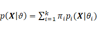 for all
 ![]() , where
, where 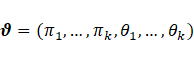 is the vector of parameters, and
 ![]() and k are the mixing proportion and
the number of mixture components, respectively, so that
and k are the mixing proportion and
the number of mixture components, respectively, so that  and
and  . Additionally,
  is referred to as the density of the
ith component. In the mixture of MVTDs, component density with a
is referred to as the density of the
ith component. In the mixture of MVTDs, component density with a ![]() mean matrix
mean matrix ![]() , two covariance matrices
, two covariance matrices ![]() and
and ![]() with dimensions
with dimensions ![]() and
and ![]() , and degrees of freedom
, and degrees of freedom ![]() is as follows [27]:
is as follows [27]:
|
|
(1) |

where T and p indicate the number of
measurement times and the number of response variables, respectively. In
addition, ![]() and
and ![]() are commonly referred to as between
and within covariance matrices, respectively. In the present study, the upper
case boldface was used for the matrices.
are commonly referred to as between
and within covariance matrices, respectively. In the present study, the upper
case boldface was used for the matrices.
The MVTDs arise as a particular case of a normal variance mixture distribution. In this formulation, the random matrix X is defined as [12]:
|
|
(2) |
where the matrix random V has the MVND
with the mean matrix 0 and covariance matrices ![]() and
and ![]() ,
, ![]() , and the latent random variable W
follows a gamma distribution with parameters
, and the latent random variable W
follows a gamma distribution with parameters ![]() . In addition,
the estimates of
. In addition,
the estimates of ![]() and
and ![]() are not unique. For each positive and
nonzero constant a, we have:
are not unique. For each positive and
nonzero constant a, we have:
|
|
(3) |
The constraint ![]() or
or ![]() can be used to obtain an identifiable
solution for
can be used to obtain an identifiable
solution for ![]() and
and ![]() (McNicholas
and Murphy, 2010; McNicholas and Subedi, 2012; Anderlucci and Viroli, 2015a;
Gallaugher and McNicholas, 2017a; Gallaugher and McNicholas, 2017b; Gallaugher
and McNicholas, 2019)
(McNicholas
and Murphy, 2010; McNicholas and Subedi, 2012; Anderlucci and Viroli, 2015a;
Gallaugher and McNicholas, 2017a; Gallaugher and McNicholas, 2017b; Gallaugher
and McNicholas, 2019)
2.2 The decomposition of covariance matrices
Restrictions on mixture parameters are typically constructed by constraining covariance matrices. Further, restrictions on mean parameters can be imposed, for example, by considering a linear model of mean parameters instead of the parameters themselves [17], [28]. To achieve parsimonious models, eigenvalue and the modified Cholesky decompositions were used for the between and within covariance matrices, respectively.
2.2.1 The eigenvalue decomposition
Celeux
and Govaert (1995), as well as Banfield
and Raftery (1993) utilized the eigenvalue decomposition in
multivariate normal mixtures. This decomposition was used for the other
multivariate mixture distributions such as t-mixture distributions [21],
along with skew-normal and skew-t mixture distributions [22]
for clustering, classification, and discriminant analysis. On the other hand, Viroli
(2011) and. Sarkar
et al. (2020) applied the
eigenvalue decomposition in the mixture of MVNDs. This parameterization
includes the expression within component-covariance matrix (![]() ) in terms of its eigenvalue
decomposition as
) in terms of its eigenvalue
decomposition as 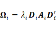 , where
 ![]() denotes the matrix of eigenvectors
Furthermore,
denotes the matrix of eigenvectors
Furthermore, ![]() is a diagonal matrix whose elements
are proportional to the eigenvalues of
is a diagonal matrix whose elements
are proportional to the eigenvalues of ![]() and
and ![]() represents the associated
proportionality constant. Different sub-models can be defined by considering
homoschedastic or varying quantities across mixture components. According to Fraley
and Raftery (2002) and Viroli
(2011), the names of eight sub-models are provided in Table 1.
represents the associated
proportionality constant. Different sub-models can be defined by considering
homoschedastic or varying quantities across mixture components. According to Fraley
and Raftery (2002) and Viroli
(2011), the names of eight sub-models are provided in Table 1.
2.2.2 Modified Cholesky decomposition
The
between component-covariance matrix (![]() ) of the multivariate longitudinal
data can be decomposed by the modified Cholesky decomposition. McNicholas
and Murphy (2010) in addition to McNicholas
and Subedi (2012) employed the
above-mentioned decomposition in clustering longitudinal data by multivariate
normal and t-mixture distributions, respectively. For multivariate longitudinal
data, Anderlucci
and Viroli, (2015a) used this decomposition, along with the
eigenvalue decomposition for the between and within covariance
structures in the mixture of MVNDs, respectively. The modified
Cholesky decomposition was expressed as
) of the multivariate longitudinal
data can be decomposed by the modified Cholesky decomposition. McNicholas
and Murphy (2010) in addition to McNicholas
and Subedi (2012) employed the
above-mentioned decomposition in clustering longitudinal data by multivariate
normal and t-mixture distributions, respectively. For multivariate longitudinal
data, Anderlucci
and Viroli, (2015a) used this decomposition, along with the
eigenvalue decomposition for the between and within covariance
structures in the mixture of MVNDs, respectively. The modified
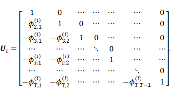
Cholesky decomposition was expressed as 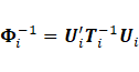 where
where ![]() is a unique
lower triangular matrix with diagonal elements 1 and
is a unique
lower triangular matrix with diagonal elements 1 and ![]() denotes a unique diagonal matrix with
strictly positive diagonal entries representing innovation variances. The
matrix
denotes a unique diagonal matrix with
strictly positive diagonal entries representing innovation variances. The
matrix ![]() has the following form:
has the following form:
|
|
)4( |
The lower diagonal elements in ![]() equal the negative coefficients resulted from the
regression of
equal the negative coefficients resulted from the
regression of ![]() on
on ![]() [32]:
[32]:
|
|
)5( |
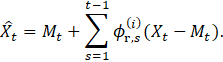
On
the other hand, different orders (m) can be considered in matrix ![]() , where m can range from 0 to T-1. The
lower orders provide more parsimonious models so that m=0 and m=1 equal the
independency of different times and the dependency of
, where m can range from 0 to T-1. The
lower orders provide more parsimonious models so that m=0 and m=1 equal the
independency of different times and the dependency of ![]() on a previous time (
on a previous time (![]() ), and the like. Accordingly, the
modified Cholesky decomposition for the temporal covariance matrix equals the
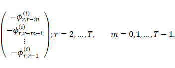
generalized autoregressive with process order m, GAR(m). Thus, the rth
row elements of matrix
), and the like. Accordingly, the
modified Cholesky decomposition for the temporal covariance matrix equals the
generalized autoregressive with process order m, GAR(m). Thus, the rth
row elements of matrix ![]() which should be estimated can be
written as follows:
which should be estimated can be
written as follows:
|
|
)6( |
Additionally, matrix ![]() can be defended as
can be defended as ![]() (Isotropic) for a more
parsimonious model. In addition, different sub-models can be defined by
considering homoschedastic or varying quantities (i.e.,
(Isotropic) for a more
parsimonious model. In addition, different sub-models can be defined by
considering homoschedastic or varying quantities (i.e., ![]() and
and ![]() ) across mixture components. Table 1
presents the names of the four sub-models for the structure of temporal
covariance according to the nomenclature of Anderlucci
and Viroli (2015a). These names
are defined based on the heteroscedastic (GAR) or homoscedastic (EGAR) of
) across mixture components. Table 1
presents the names of the four sub-models for the structure of temporal
covariance according to the nomenclature of Anderlucci
and Viroli (2015a). These names
are defined based on the heteroscedastic (GAR) or homoscedastic (EGAR) of ![]() and the isotropic of
and the isotropic of ![]() .
.
Table 1:Parsimonious within and temporal covariance structures, descriptions and number of parameters
|
|
Descriptions |
Components |
Number of parameters |
||
|
|
|
|
|
|
|
|
VVV |
Heteroscedastic components |
|
|
|
|
|
EEV |
Ellipsoidal, equal volume and equal space |
|
|
|
|
|
EEE |
Homoscedastic components |
|
|
|
|
|
III |
Spherical components with unit volume |
|
|
|
|
|
VVI |
Diagonal but varying variability components |
|
|
|
|
|
EEI |
Diagonal and homoscedastic components |
|
|
|
|
|
VII |
Spherical components with varying volume |
|
|
|
|
|
EII |
Spherical components without varying volume |
|
|
|
|
|
|
|
|
|
||
|
GAR(m) |
Heteroscedastic components |
|
|
|
|
|
GARI(m) |
GAR + Isotropic for |
|
|
|
|
|
EGAR(m) |
Homoscedastic components |
|
|
|
|
|
EGARI(m) |
EGAR+ Isotropic for |
|
|
|
|
![]()
![]() : The
number of
: The
number of ![]() parameters
parameters
3. Method
3.1 Estimation of parameters
To find the maximum likelihood estimators for mixture parameters, the present study used an expectation-maximization (EM) algorithm for the mixture of matrix-variate t-distributions (MVTDs).
Assume that ![]() , where n is the number of
observations, be a random sample of matrices from the mixture of MVTDs, and
, where n is the number of
observations, be a random sample of matrices from the mixture of MVTDs, and ![]() denotes the component membership of
observation j. Further,
denotes the component membership of
observation j. Further, ![]() if the jth observation is
from component i, otherwise,
if the jth observation is
from component i, otherwise, ![]() , where
, where ![]() and
and ![]() . Based on the
representation of normal-variance mixture, MVTDs
are expressed as follows:
. Based on the
representation of normal-variance mixture, MVTDs
are expressed as follows:
|
|
(7) |
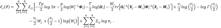
Based on the hierarchical
representation of the MVTDs, the
complete data log-likelihood ![]() can be written as follows:
can be written as follows:
|
|
(8) |
An EM algorithm is as follows:
I.
Initialization: Initialize parameters ![]() ,
, ![]() ,
, ![]() ,
, ![]() , and
, and ![]() , setting
, setting ![]() .
.
II. E-step: Update ![]() ,
, ![]() , and
, and ![]() , where
, where
|
|
(9) |
|
|
(10) |
|
|
(11) |
where
![]() represents the
digamma function. Furthermore,
represents the
digamma function. Furthermore, ![]() is calculated based on
is calculated based on ![]() distribution, which has a
gamma distribution with parameters
distribution, which has a
gamma distribution with parameters ![]() , and
, and ![]() is achieved using the
moment-generating function of
is achieved using the
moment-generating function of ![]() .
.
III.
M-step: Update ![]() ,
, ![]() ,
, ![]() ,
, ![]() , and
, and ![]() . The order of parameter estimation is as follows
(1):
. The order of parameter estimation is as follows
(1): ![]() and
and ![]() ; (2)
; (2) ![]() ; (3)
; (3) ![]() ; (4)
; (4) ![]()
1.
Update ![]() and
and ![]()
|
|
(12) |
2.
Update ![]()
Assuming that ![]() , the
, the ![]() is proportional to
is proportional to ![]() with
with ![]() . The estimates o parameters for the
eight sub-models are provided below.
. The estimates o parameters for the
eight sub-models are provided below.
·
Sub-model VVV:
The maximization of  with respect to
 ![]() leads to
leads to 
·
Sub-model EEE:
The maximization of  , where
  , with respect to
 ![]() leads to
leads to 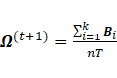 ;
;
·
Sub-model VVI: The maximization of ![]() with respect to
with respect to ![]() leads to
leads to ![]() and
and![]() ;
;
·
Sub-model EEI:
The maximization of 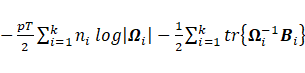 with respect to
  leads to
 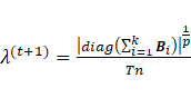 and
and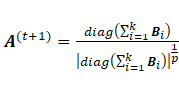 ;
;
·
Sub-model VII:
The maximization of 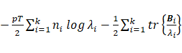 with respect to
  leads to
 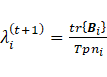 ;
;
·
Sub-model EII:
The maximization of 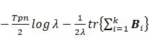 with respect to
  leads to
 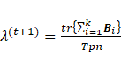 ;
;
·
Sub-model EEV: The maximization of ![]() with respect to
with respect to ![]() leads to
leads to 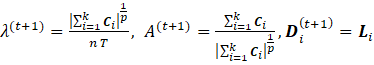 , where for
 ![]()
![]() , and
, and ![]() are derived from the eigenvalue decomposition of the symmetric
positive definite matrix
are derived from the eigenvalue decomposition of the symmetric
positive definite matrix ![]()
![]() with the eigenvalues in the diagonal matrix
with the eigenvalues in the diagonal matrix ![]() in descending order.
in descending order.
· Sub-model III: This situation equals the independence of the responses thus no parameters are available.
Further
estimation details related to the covariance matrix ![]() are provided in (Celeux
and Govaert, 1995; Viroli, 2011; L Anderlucci and Viroli, 2015a; Sarkar et
al., 2020).
are provided in (Celeux
and Govaert, 1995; Viroli, 2011; L Anderlucci and Viroli, 2015a; Sarkar et
al., 2020).
3. Update ![]()
Considering that ![]() is proportional to
is proportional to ![]() . The
estimates of parameters for the four sub-models are presented as follows:
. The
estimates of parameters for the four sub-models are presented as follows:
·
Sub-model GAR(m): The
maximization of 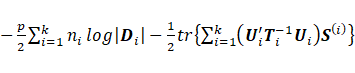 with respect to
 ![]() leads to the rth
row estimation of matrix
leads to the rth
row estimation of matrix ![]() as
as
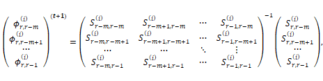
and
matrix![]() , where
, where ![]() and
and ![]() is the lth-row
and rth-column element of matrix
is the lth-row
and rth-column element of matrix ![]() .
.
·
Sub-model GARI(m): The maximization of ![]() with respect to
with respect to ![]() leads to the same estimate of
leads to the same estimate of ![]() as sub-model GAR(m) and estimate
as sub-model GAR(m) and estimate ![]() .
.
·
Sub-model EGAR(m): The maximization of ![]() with respect to
with respect to ![]() leads to the same estimate of
leads to the same estimate of ![]() as sub-model GAR(m) by replacing
as sub-model GAR(m) by replacing ![]() instead of
instead of ![]() and estimate
and estimate ![]() .
.
·
Sub-model EGARI(m): The maximization of ![]() with respect to
with respect to ![]() leads to the same estimate of
leads to the same estimate of ![]() as sub-model EGAR(m) and estimate
as sub-model EGAR(m) and estimate ![]() .
.
Refer to (McNicholas
and Murphy, 2010; McNicholas and Subedi, 2012; Anderlucci and Viroli, 2015a)
for further details on the estimation of the covariance matrix ![]() .
.
4. Update ![]()
For the degree
of freedom, two situations were considered,
including equal and unequal ![]() across mixture components
(constrained and unconstrained
across mixture components
(constrained and unconstrained ![]() respectively). Given
respectively). Given ![]() ,
, ![]() ,
, ![]() ,
, ![]() , and
, and ![]() , the
estimations of
, the
estimations of ![]() are calculated
by finding the root of equations (13) and (14) in constrained and unconstrained
situations, respectively.
are calculated
by finding the root of equations (13) and (14) in constrained and unconstrained
situations, respectively.
|
|
(13) |
|
|
(14) |
IV. Check the
convergence criterion: If not satisfied, set ![]() and go to step II of the EM algorithm iteration.
and go to step II of the EM algorithm iteration.
3.2 Model selection and convergence criterion
It
is possible to define a large family (![]() ) of possible
mixture models by allowing different sub-models for covariance matrices
) of possible
mixture models by allowing different sub-models for covariance matrices ![]() and
and ![]() with different orders for matrix
with different orders for matrix ![]() ,
,  , and constrained/unconstrained for
 ![]() . The model can be selected according
to the Bayesian information criterion (BIC) as follows [33]:
. The model can be selected according
to the Bayesian information criterion (BIC) as follows [33]:
|
|
)15( |
where
![]() and
and ![]() indicate
the maximized log-likelihood and the maximum likelihood estimate of
indicate
the maximized log-likelihood and the maximum likelihood estimate of ![]() , respectively. Additionally,
, respectively. Additionally, ![]() and
n are the number of free parameters in the model and the number of
observations, respectively.
and
n are the number of free parameters in the model and the number of
observations, respectively.
Other criteria are employed in addition to BIC to estimate the number of mixture components, such as Integrated Completed Likelihood (ICL), which is computed as follows [34]:
|
|
)16( |
where MAP (τij(t)) )=1 if the maxi=1,…,k {τij(t)}=i, otherwise, MAP(τij(t))=0, j=1 ,…,n and i=1,…,k.
In
general, 20 random multistate points were considered given that the starting
values of the EM algorithm could affect the estimated parameters. If
the convergence criterion ![]() is met, the EM algorithm is stopped,
and the range of values for
is met, the EM algorithm is stopped,
and the range of values for ![]() is limited to between 2 and 200 [21].
These models have been written in R and are accessible on request.
is limited to between 2 and 200 [21].
These models have been written in R and are accessible on request.
3.3 Calculate the standard error of parameters
The observed
information matrix may be used to calculate the parameter's standard error. The
observed information matrix is computed as ![]() , where
, where ![]() is the Hessian matrix of the
likelihood function for observation j. The hessian function in numDeriv
package in R software could be used to calculate
is the Hessian matrix of the
likelihood function for observation j. The hessian function in numDeriv
package in R software could be used to calculate ![]() (Anderlucci
and Viroli, 2015a).
(Anderlucci
and Viroli, 2015a).
4. Simulation studies and real data
4.1 Simulation 1
The
first simulation study was conducted to evaluate the
ability of the algorithm for recognizing the temporal structure. The
features of simulation study 1 were: a
number k of mixture components equal to 3, a
k-vector of the degrees of freedom equal to 5, 5, 5, and a 4
![]() 4 within covariance matrix
4 within covariance matrix ![]() with a structure equals to VVV. In
addition, other features included a 6
with a structure equals to VVV. In
addition, other features included a 6![]() 6 temporal covariance matrix
6 temporal covariance matrix ![]() with a structure equals to GAR(1) and
GAR(3), and a sample size n equals 100, 200, 500, and 1000. For
each setting, 100 datasets were generated from the mixture of the MVTDs based
on the defined within and temporal covariance matrices. Then,
the mixture of MVTDs and MVNDs was run for five different models according to
different orders for
with a structure equals to GAR(1) and
GAR(3), and a sample size n equals 100, 200, 500, and 1000. For
each setting, 100 datasets were generated from the mixture of the MVTDs based
on the defined within and temporal covariance matrices. Then,
the mixture of MVTDs and MVNDs was run for five different models according to
different orders for ![]() : GAR(1), GAR(2), GAR(3), GAR(4), and
GAR(5). The best model was chosen according to the BIC and ICL. Table 2
contains the number of times a model with GAR(1) and GAR(3) structures for
: GAR(1), GAR(2), GAR(3), GAR(4), and
GAR(5). The best model was chosen according to the BIC and ICL. Table 2
contains the number of times a model with GAR(1) and GAR(3) structures for ![]() was selected as the best model based
on the BIC and ICL. To converge the EM algorithm, MVTD models with the
constrained degrees of freedom were fitted in settings with the
GAR(3) true structure and the sample sizes of 100 and 200 while MVTD models
with unconstrained degrees of freedom were run in
other settings.
was selected as the best model based
on the BIC and ICL. To converge the EM algorithm, MVTD models with the
constrained degrees of freedom were fitted in settings with the
GAR(3) true structure and the sample sizes of 100 and 200 while MVTD models
with unconstrained degrees of freedom were run in
other settings.
The percentage (number) of correct model selection with MVTD is equal to 100 in all cases, and it ranges from 97 to 100 for MVNDs. In a situation with a true model GAR(3), this percentage varied from 99 to 100 and 93 to 99 for MVTD and MVND, respectively.
Table
2: The number of times a model with GAR(1) or GAR(3) structure for ![]() was chosen according to the BIC and ICL
criterion, from the simulation 1
was chosen according to the BIC and ICL
criterion, from the simulation 1
|
n |
|
|
|||||
|
GAR(1) |
GAR(2) |
GAR(3) |
GAR(4) |
GAR(5) |
|||
|
Model |
True Sub-model: GAR(1) |
||||||
|
100 |
MVTD |
100 |
0 |
0 |
0 |
0 |
|
|
MVND |
97 |
3 |
0 |
0 |
0 |
||
|
200 |
MVTD |
100 |
0 |
0 |
0 |
0 |
|
|
MVND |
99 |
1 |
0 |
0 |
0 |
||
|
500 |
MVTD |
100 |
0 |
0 |
0 |
0 |
|
|
MVND |
100 |
0 |
0 |
0 |
0 |
||
|
1000 |
MVTD |
100 |
0 |
0 |
0 |
0 |
|
|
MVND |
99 |
1 |
0 |
0 |
0 |
||
|
|
True Sub-model: GAR(3) |
||||||
|
100 |
MVTD |
0 |
0 |
97 |
2 |
1 |
|
|
MVND |
1 |
0 |
93 |
4 |
2 |
||
|
200 |
MVTD |
0 |
0 |
100 |
0 |
0 |
|
|
MVND |
0 |
1 |
95 |
3 |
1 |
||
|
500 |
MVTD |
0 |
0 |
100 |
0 |
0 |
|
|
MVND |
0 |
0 |
98 |
1 |
1 |
||
|
1000 |
MVTD |
0 |
0 |
100 |
0 |
0 |
|
|
MVND |
0 |
0 |
99 |
1 |
0 |
||
4.2 Simulation 2
It
is known that t-distributions can recover normal distributions by estimating
larger values of the degrees of freedom parameters. Further, t-distribution
mixture models can be used when mixture components are derived from normal and
t-distributions. The simulation study 2 was performed to evaluate the ability
of MVTDs to recover the MVNDs in multivariate longitudinal data. To this end,
datasets were generated from two-component (k=2), matrix-variate mixture
models. The MVND and MVTD were the first and second components, respectively,
and the same covariance structures with different parameter values were used
accordingly. Other features (i.e., ![]() ,
, ![]() , and sample size) in
this simulation are similar to the first simulation study. For each setting,
100 datasets were generated from mixture distributions based on the defined within
and temporal covariance matrices. Further, the mixture of MVTDs and MVNDs was
run for five different models of GAR(1), GAR(2), GAR(3), GAR(4), and GAR(5).
Table 3 presents the average values of the degree of freedom (standard
deviation) of a model with GAR(1) and GAR(3) structures for
, and sample size) in
this simulation are similar to the first simulation study. For each setting,
100 datasets were generated from mixture distributions based on the defined within
and temporal covariance matrices. Further, the mixture of MVTDs and MVNDs was
run for five different models of GAR(1), GAR(2), GAR(3), GAR(4), and GAR(5).
Table 3 presents the average values of the degree of freedom (standard
deviation) of a model with GAR(1) and GAR(3) structures for ![]() . Based on the obtained data, the
sample size of 100 was not considered for a setting with the GAR(3) true
temporal due to the lack of convergence of the EM algorithm. Given k (=2) and
. Based on the obtained data, the
sample size of 100 was not considered for a setting with the GAR(3) true
temporal due to the lack of convergence of the EM algorithm. Given k (=2) and ![]() (VVV), the estimated degrees of
freedom demonstrated that the first component was normal. Furthermore, the
degrees of freedom estimates were computed to be close to true values in MVTD
mixture models.
(VVV), the estimated degrees of
freedom demonstrated that the first component was normal. Furthermore, the
degrees of freedom estimates were computed to be close to true values in MVTD
mixture models.
Based on Tables 3 and 5, the true model GAR(3) had a worse performance compared to the true model GAR(1). Therefore, the results related to the simulation studies of the true model GAR(3) are presented in the continuation.
Additionally, the misclassification error rate
(MISC) and the measure of accuracy (![]() ) for mean and covariance matrices
were computed for each dataset and model in order to compare the two models in
parameter estimates. Therefore, the accuracy measures of
) for mean and covariance matrices
were computed for each dataset and model in order to compare the two models in
parameter estimates. Therefore, the accuracy measures of ![]() ,
, ![]() (=VVV),
(=VVV), ![]() , and
, and ![]() (=GAR) were calculated by the
following expressions (Anderlucci
and Viroli, 2015b):
(=GAR) were calculated by the
following expressions (Anderlucci
and Viroli, 2015b):
|
|
)17( |
where the
lower accuracy measure (![]() ) implies higher accuracy for
parameters.
) implies higher accuracy for
parameters.
Table 4 provides the average (standard deviation)
values of MISC and the accuracy measures of a model with GAR(3) for ![]() . Considering k
(=2) and
. Considering k
(=2) and ![]() (VVV), the accuracy measures (
(VVV), the accuracy measures (![]() ,
, ![]() , and
, and ![]() ) were not sensitive to the
misspecification of the order of the temporal covariance (m=1, 2, …, 5), and
these values were nearly identical in MVTD and MVND mixture models. However,
the values of the accuracy measure (
) were not sensitive to the
misspecification of the order of the temporal covariance (m=1, 2, …, 5), and
these values were nearly identical in MVTD and MVND mixture models. However,
the values of the accuracy measure (![]() ) relied on the misspecification of
the temporal covariance order. In the two models, the accuracy measure
) relied on the misspecification of
the temporal covariance order. In the two models, the accuracy measure ![]() ) of the lower orders (
) of the lower orders (![]() ) was larger compared to the higher
orders (
) was larger compared to the higher
orders (![]() ). It should be noted that MVND
mixture models tend to overestimate the accuracy measure (
). It should be noted that MVND
mixture models tend to overestimate the accuracy measure (![]() ) compared to MVTD mixture models.
Eventually, the accuracy measures in both models decreased by an increase in
the sample size. The mean compute time for fitting the mixture of MVTDs vs as
MVNDs with the true model GAR(3) was 6.66 vs. 0.37 for n=100, 10.17 vs. 0.62
for n=200, 23.44 vs. 1.30 for n=500, and 46.86 vs 2.59 for n=1000.
) compared to MVTD mixture models.
Eventually, the accuracy measures in both models decreased by an increase in
the sample size. The mean compute time for fitting the mixture of MVTDs vs as
MVNDs with the true model GAR(3) was 6.66 vs. 0.37 for n=100, 10.17 vs. 0.62
for n=200, 23.44 vs. 1.30 for n=500, and 46.86 vs 2.59 for n=1000.
Table
3: Mean (S.D) of degree of freedom with GAR(1) or GAR(3) structure
for ![]() from simulation 2
from simulation 2
|
n |
|
||||
|
GAR(1) |
GAR(2) |
GAR(3) |
GAR(4) |
GAR(5) |
|
|
True Sub-model: GAR(1) |
|||||
|
100 |
174.9 (48.2) |
175.6 (46.5) |
176.3 (45.6) |
176.7 (45.2) |
177.4 (45.6) |
|
5.42 (1.30) |
5.42 (1.32) |
5.43 (1.31) |
5.43 (1.30) |
5.43 (1.30) |
|
|
200 |
189.4 (30.1) |
189.3 (30.4) |
189.8 (29.6) |
189.9 (29.5) |
190.2 (29.2) |
|
5.09 (0.79) |
5.09 (0.79) |
5.09 (0.79) |
5.10 (0.79) |
5.10 (0.78) |
|
|
500 |
192.0 (23.3) |
191.9 (23.2) |
192.4 (22.7) |
192.6 (22.4) |
192.6 (22.3) |
|
5.05 (0.51) |
5.05 (0.51) |
5.05 (0.51) |
5.05 (0.51) |
5.05 (0.51) |
|
|
1000 |
199.6 (3.9) |
199.6 (3.7) |
199.7 (3.3) |
199.7 (2.9) |
199.7 (2.6) |
|
4.99 (0.35) |
4.99 (0.35) |
4.99 (0.35) |
4.99 (0.35) |
4.99 (0.35) |
|
|
|
True Sub-model: GAR(3) |
||||
|
200 |
175.8 (48.6) |
160.8 (31.5) |
189.3 (31.2) |
189.7 (30.8) |
189.9 (30.4) |
|
4.75 (0.84) |
4.77 (0.85) |
5.09 (0.87) |
5.10(0.88) |
5.10 (0.88) |
|
|
500 |
116.2 (44.3) |
167.1 (42.9) |
195.0 (19.7) |
195.1(19.6) |
195.1 (19.6) |
|
4.74 (0.43) |
4.85 (0.43) |
5.06 (0.43) |
5.07(0.43) |
5.07 (0.43) |
|
|
1000 |
119.6 (41.9) |
178.7 (34.2) |
198.2 (9.3) |
198.2(9.2) |
198.2 (9.2) |
|
4.70 (0.38) |
4.97 (0.39) |
5.05 (0.41) |
5.05(0.41) |
5.05 (0.41) |
|
Table
4: Mean (S.D) of MISC and accuracy measures with GAR(3) structure for ![]() from simulation 2
from simulation 2
|
|
|
Model |
|
||||
|
n |
|
GAR(1) |
GAR(2) |
GAR(3) |
GAR(4) |
GAR(5) |
|
|
200 |
MISC |
MVTD |
0 |
0 |
0 |
0 |
0 |
|
MVND |
0.0001(0.001) |
0.0001(0.001) |
0.0001(0.001) |
0.0001(0.001) |
0.0001(0.001) |
||
|
|
MVTD |
0.09 (0.01) |
0.09 (0.01) |
0.09 (0.01) |
0.09 (0.01) |
0.09 (0.01) |
|
|
MVND |
0.10 (0.01) |
0.10 (0.01) |
0.10 (0.01) |
0.10 (0.01) |
0.10 (0.01) |
||
|
|
MVTD |
0.23 (0.002) |
0.23 (0.001) |
0.23 (0.001) |
0.23 (0.001) |
0.23 (0.001) |
|
|
MVND |
0.23 (0.003) |
0.23 (0.002) |
0.23 (0.001) |
0.23 (0.001) |
0.23 (0.001) |
||
|
|
MVTD |
0.49 (0.02) |
0.44 (0.02) |
0.40 (0.02) |
0.40 (0.02) |
0.40 (0.02) |
|
|
MVND |
0.57 (0.06) |
0.52 (0.13) |
0.48 (0.14) |
0.48 (0.14) |
0.48 (0.14) |
||
|
|
MVTD |
0.33 (0.002) |
0.20 (0.01) |
0.10 (0.02) |
0.15 (0.04) |
0.18 (0.04) |
|
|
MVND |
0.33 (0.002) |
0.20 (0.02) |
0.11 (0.03) |
0.17 (0.05) |
0.21 (0.06) |
||
|
500 |
MISC |
MVTD |
0 |
0 |
0 |
0 |
0 |
|
MVND |
0 |
0 |
0 |
0 |
0 |
||
|
|
MVTD |
0.08 (0.01) |
0.08 (0.01) |
0.08 (0.01) |
0.08 (0.01) |
0.08 (0.01) |
|
|
MVND |
0.09 (0.01) |
0.09 (0.01) |
0.09 (0.01) |
0.09 (0.01) |
0.09 (0.01) |
||
|
|
MVTD |
0.18 (0.0003) |
0.18 (0.0002) |
0.18 (0.0002) |
0.18 (0.0002) |
0.18 (0.0002) |
|
|
MVND |
0.18 (0.0003) |
0.18 (0.0003) |
0.18 (0.0003) |
0.18 (0.0003) |
0.18 (0.0003) |
||
|
|
MVTD |
0.47 (0.01) |
0.38 (0.01) |
0.35 (0.01) |
0.35 (0.01) |
0.35 (0.01) |
|
|
MVND |
0.51 (0.02) |
0.45 (0.02) |
0.41 (0.02) |
0.41 (0.02) |
0.41 (0.02) |
||
|
|
MVTD |
0.30 (0.002) |
0.19 (0.004) |
0.08 (0.01) |
0.08 (0.01) |
0.08 (0.01) |
|
|
MVND |
0.30 (0.003) |
0.19 (0.004) |
0.09 (0.01) |
0.09 (0.01) |
0.09 (0.01) |
||
|
1000 |
MISC |
MVTD |
0 |
0 |
0 |
0 |
0 |
|
MVND |
0 |
0 |
0 |
0 |
0 |
||
|
|
MVTD |
0.06 (0.01) |
0.06 (0.01) |
0.06 (0.01) |
0.06 (0.01) |
0.06 (0.01) |
|
|
MVND |
0.07 (0.01) |
0.07 (0.01) |
0.07 (0.01) |
0.07 (0.01) |
0.07 (0.01) |
||
|
|
MVTD |
0.15 (0.0002) |
0.15 (0.0002) |
0.15 (0.0002) |
0.15 (0.0002) |
0.15 (0.0002) |
|
|
MVND |
0.15 (0.0002) |
0.15 (0.0002) |
0.15 (0.0002) |
0.15 (0.0002) |
0.15 (0.0002) |
||
|
|
MVTD |
0.31 (0.01) |
0.27 (0.01) |
0.27 (0.01) |
0.27 (0.01) |
0.27 (0.01) |
|
|
MVND |
0.42 (0.03) |
0.40 (0.02) |
0.37 (0.02) |
0.37 (0.02) |
0.37 (0.02) |
||
|
|
MVTD |
0.28 (0.001) |
0.17 (0.001) |
0.05 (0.001) |
0.05 (0.001) |
0.05 (0.001) |
|
|
MVND |
0.28 (0.001) |
0.20 (0.001) |
0.06 (0.01) |
0.06 (0.01) |
0.06 (0.01) |
||
4.3 Simulation 3
The number of components was considered constant and the mixture models were fitted in the two preceding simulation studies. In the third simulation study, the ability of MVTD and the MVND mixture models was evaluated regarding recognizing the true number of mixture components when the data were generated from MVTD mixture models. Then, the impact of the misspecification of the temporal matrix on the estimation of the number of components was investigated as well. The same parameters were used in this simulation as in the first simulation.
For each setting, 100 datasets were generated from the model with a GAR(3) structure. In addition, a different number of mixture components (k = 2, 3, and 4) was considered to evaluate the choice of k. Table 5 presents the number of times a model with a particular number of mixture components was chosen as the best model in each of the five different models of GAR(1), GAR(2), GAR(3), GAR(4), and GAR(5). Approximately the correct number of components (k=3) was selected for MVTDs in all cases. However, MVNDs tend to overestimate (k=4) the number of true components. As the sample size increased, the correct number of components reached 100 in MVTD, while it was completely overestimated in MVND. Also, in a small sample size (n=200), the ability to detect the correct number of components increased with the increase of m in both models.
Table
5: The number of times a model with the true number of component
(k=3) and GAR(3) structure for ![]() for the different temporal structures
was chosen from simulation 3
for the different temporal structures
was chosen from simulation 3
|
n |
Model |
k |
True Sub-model: GAR(3) |
||||
|
GAR(1) |
GAR(2) |
GAR(3) |
GAR(4) |
GAR(5) |
|||
|
200 |
MVTD |
2 |
0 |
0 |
0 |
0 |
0 |
|
3 |
95 |
99 |
96 |
100 |
100 |
||
|
4 |
5 |
1 |
4 |
0 |
0 |
||
|
MVND |
2 |
0 |
0 |
0 |
0 |
0 |
|
|
3 |
42 |
53 |
62 |
68 |
73 |
||
|
4 |
58 |
47 |
38 |
32 |
27 |
||
|
500 |
MVTD |
2 |
0 |
0 |
0 |
0 |
0 |
|
3 |
100 |
100 |
100 |
100 |
100 |
||
|
4 |
0 |
0 |
0 |
0 |
0 |
||
|
MVND |
2 |
0 |
0 |
0 |
0 |
0 |
|
|
3 |
0 |
0 |
0 |
0 |
0 |
||
|
4 |
100 |
100 |
100 |
100 |
100 |
||
|
1000 |
MVTD |
2 |
0 |
0 |
0 |
0 |
0 |
|
3 |
100 |
100 |
100 |
100 |
100 |
||
|
4 |
0 |
0 |
0 |
0 |
0 |
||
|
MVND |
2 |
0 |
0 |
0 |
0 |
0 |
|
|
3 |
0 |
0 |
0 |
0 |
0 |
||
|
4 |
100 |
100 |
100 |
100 |
100 |
||
4.4 Real data: Gastrointestinal (GI) cancers
The age-standardized death rates of the three
most common GI cancers were extracted from the Our World In Data website
[36].
The information included the death rates (per 100,000 populations)
of colon and rectum, stomach, and liver cancers in 186 countries during
1990-2015 (at 5-year intervals), ![]() is a matrix with
dimension
is a matrix with
dimension ![]() . A mixture of MVTDs and MVNDs was
fitted with k ranging from 1 to 10. The best sub-model based on the BIC
and ICL is (GAR(2), VVV) with k=7 in the mixture of MVNDs and (GAR(4),
VVV) with the constrained degrees of freedom and k=6 in the mixture of MVTDs
(Table 6). The estimated degree of freedom for the mixture of the MVTDs
was
. A mixture of MVTDs and MVNDs was
fitted with k ranging from 1 to 10. The best sub-model based on the BIC
and ICL is (GAR(2), VVV) with k=7 in the mixture of MVNDs and (GAR(4),
VVV) with the constrained degrees of freedom and k=6 in the mixture of MVTDs
(Table 6). The estimated degree of freedom for the mixture of the MVTDs
was ![]() . Further, stomach and
liver cancer death rates in some countries were extremely higher
compared to other countries. Thus, the mixture of the MVND model provided an
additional cluster to allow outliers.
. Further, stomach and
liver cancer death rates in some countries were extremely higher
compared to other countries. Thus, the mixture of the MVND model provided an
additional cluster to allow outliers.
Table 6: Results of the mixture of the MVTD and MVND models for the three common GI cancers
|
Model |
BIC |
ICL |
|
|
m |
k |
|
RMSD |
Compute time for fitting (Second) |
|
MVTD |
9275.63 |
9240.58 |
VVV |
GAR |
4 |
6 |
3.33 |
9.42 |
165.42 |
|
MVND |
9666.63 |
9683.78 |
VVV |
GAR |
2 |
7 |
- |
11.20 |
127.80 |
Table 7: Estimated component means of the countries based on the death rates of the three common GI cancers resulted from the mixture of the MVTD models
|
Year |
k |
Type of cancer |
|||||
|
2015 |
2010 |
2005 |
2000 |
1995 |
1990 |
||
|
9.75 |
9.53 |
9.25 |
9.98 |
8.89 |
8.69 |
1 |
Colon and rectum |
|
8.96 |
8.86 |
8.83 |
8.86 |
8.61 |
8.44 |
2 |
|
|
9.67 |
9.60 |
9.59 |
9.54 |
9.47 |
9.12 |
3 |
|
|
8.35 |
8.29 |
8.21 |
8.10 |
7.83 |
7.73 |
4 |
|
|
16.53 |
17.23 |
18.01 |
16.98 |
18.30 |
15.89 |
5 |
|
|
15.37 |
16.23 |
17.05 |
17.86 |
18.50 |
18.47 |
6 |
|
|
6.38 |
6.34 |
6.43 |
6.51 |
6.79 |
6.68 |
1 |
Liver |
|
4.27 |
4.25 |
4.37 |
4.49 |
4.44 |
4.35 |
2 |
|
|
8.60 |
8.87 |
9.34 |
9.83 |
10.01 |
9.55 |
3 |
|
|
17.63 |
18.55 |
20.03 |
21.00 |
22.52 |
21.89 |
4 |
|
|
3.60 |
3.61 |
3.67 |
3.20 |
3.58 |
2.96 |
5 |
|
|
4.35 |
4.23 |
4.15 |
4.12 |
4.02 |
3.84 |
6 |
|
|
13.05 |
14.13 |
15.48 |
16.85 |
18.87 |
20.22 |
1 |
Stomach |
|
6.04 |
6.43 |
7.01 |
7.83 |
8.37 |
8.82 |
2 |
|
|
8.32 |
9.98 |
9.74 |
10.78 |
11.72 |
12.10 |
3 |
|
|
12.09 |
12.66 |
12.90 |
13.15 |
13.78 |
14.99 |
4 |
|
|
12.90 |
14.98 |
17.77 |
19.21 |
24.79 |
25.23 |
5 |
|
|
6.16 |
6.91 |
7.78 |
9.08 |
10.75 |
12.49 |
6 |
|
We
also fitted a finite mixture of skew matrix-variate distributions introduced by
Gallaugher and McNicholas (2017b) to GI data. These matrix-variate
distributions are skew-t, generalized hyperbolic, variance-gamma, and normal
inverse Gaussian distributions that we did not consider eigenvalue and the
modified Cholesky decompositions for the between and within
covariance matrices for those, respectively. Because of the huge number of
parameters, any of these finite mixture had not been converge. Given k, the
number of parameters in these skew matrix-variates is  to greater than the matrix-varieties
distributions.
to greater than the matrix-varieties
distributions.
The root mean square deviation (RMSD), the quadratic mean of the differences between the observed values and predicted values, values for the mixture of MVNDs and MVTDs were 11.20 and 9.42, respectively (Table 6). For more details, maps of the included countries in each cluster of MVTD and MVND models are presented in Figures 1 and 2, respectively. The estimated component mean for each cluster of MVTD models is shown in Table 7. The colon and rectum, liver, and stomach cancer death rates were growing, nearly stable, and decreasing in the first cluster countries, respectively. The behaviour of the countries in the second and third clusters was similar to the first cluster, with the exception that the rate of decrease in liver cancer in the second cluster was slower, and the rate in the third cluster was between the first and second clusters. The fourth cluster countries' patterns are identical to the second cluster, although the decline in the liver is quicker. The colon and rectum and liver are growing in fifth cluster countries, whereas the stomach is dropping (with the highest rate of decrease among the clusters). Countries in the sixth cluster behaved similarly to those in the fifth, with the exception that the rate of change in the colon and rectum was quicker. According to Figure 2, the second cluster countries, which mostly include African and Arab countries, have the lowest death rates in the three cancers.
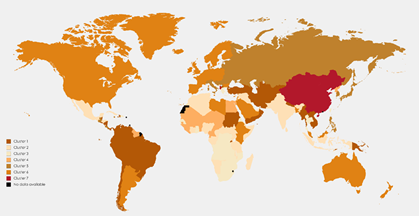
Figure 1: Map of clustering countries based on the death rates of the three common GI cancer resulted from the mixture of the MVNDs
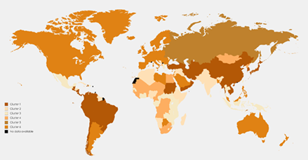
Figure 2: Map of clustering countries based on the death rates of the three common GI cancer resulted from the mixture of the MVTDs
5. Conclusion
In the present study, a family of finite matrix-variate t-distributions was evaluated for clustering multivariate longitudinal datasets. To this end, two types of constraints were utilized for covariance structures, including the eigenvalue and modified Cholesky decompositions for the within and temporal covariance matrices, respectively.
Based on accuracy measures (![]() ) in the mixture models of MVTD and
the MVND, no differences were observed between the estimation of
) in the mixture models of MVTD and
the MVND, no differences were observed between the estimation of ![]() ,
, ![]() , and
, and ![]() matrices under different orders of
temporal covariance structures in each model in simulation studies. Further,
these values were similar in both models. On the other hand, the estimation of
matrix
matrices under different orders of
temporal covariance structures in each model in simulation studies. Further,
these values were similar in both models. On the other hand, the estimation of
matrix ![]() relies on the misspecification of
relies on the misspecification of ![]() . Thus, the accuracy measure
. Thus, the accuracy measure ![]() s should have the least value compared
to lower orders if the order of the incorrect temporal structure
is equal to or greater than the correct order of the temporal structure. The
estimations of matrix T and the number of mixture components k
are overestimated in MVND models if the datasets have a heavy-tail or
outlier observations. These properties were demonstrated by McNicholas
and Subedi (2012) in the clustering of longitudinal data using the
mixture of multivariate t-distributions. On the other hand, the
time it took to fit a mixture of MVTDs was much longer than it required to fit
a mixture of MVNDs, which is a trade-off for more precision.
s should have the least value compared
to lower orders if the order of the incorrect temporal structure
is equal to or greater than the correct order of the temporal structure. The
estimations of matrix T and the number of mixture components k
are overestimated in MVND models if the datasets have a heavy-tail or
outlier observations. These properties were demonstrated by McNicholas
and Subedi (2012) in the clustering of longitudinal data using the
mixture of multivariate t-distributions. On the other hand, the
time it took to fit a mixture of MVTDs was much longer than it required to fit
a mixture of MVNDs, which is a trade-off for more precision.
The mixture of MVTDs commonly selected the model with the right temporal structure and the right number of mixture components. Based on the MISC and accuracy measures, a perfect separation was found between the mixture components and the good accuracy of parameter estimation in this mixture model. The results of these simulation studies regarding evaluating different abilities of the finite mixtures of MVTDs were similar to those of simulations in the finite mixture of the MVNDs (Anderlucci and Viroli, 2015b).
The age-standardized death rates of the three most common GI cancers (i.e., colon and rectum, stomach, and liver) from 186 countries were clustered between 1990 and 2015 (a 5-year interval) using the mixture of MVTD and MVND models. Based on the BIC and ICL, the same within and temporal covariance structures were selected in both models although the order of the temporal structure was higher in the MVTD mixture. On the other hand, one more component was available in the MVTD mixture for including outlier death rates. Based on the BIC and ICL and RMSD, MVTD mixture models better fitted to the clustering death rates of the three common GI cancers of the countries compared to MVND mixture models.
Finally, the large value of the RMSD revealed that other matrix-variate distributions (i.e., asymmetric matrix-variate distributions) could be appropriate in this regard. In our future work, we will consider the parsimonious covariance of the finite mixture of skewed matrix-variate distributions for the clustering three-way data.
References
[1] G. J. McLachlan and D. Peel, Finite mixture models. New York (NY): John Wiley & Sons, 2000. View Article
[2] P. D. McNicholas, Mixture model-based classification, 1st ed. Chapman & Hall/CRC, 2016. View Article
[3] D. Peel and G. J. McLachlan, “Robust mixture modelling using the t distribution,” Stat. Comput., vol. 10, no. 4, pp. 339–348, 2000. View Article
[4] T. I. Lin, “Maximum likelihood estimation for multivariate skew normal mixture models,” J. Multivar. Anal., vol. 100, no. 2, pp. 257–265, Feb. 2009. View Article
[5] T. I. Lin, “Robust mixture modeling using multivariate skew t distributions,” Stat. Comput., vol. 20, no. 3, pp. 343–356, Jul. 2010. View Article
[6] A. O’Hagan, T. B. Murphy, I. C. Gormley, P. D. McNicholas, and D. Karlis, “Clustering with the multivariate normal inverse Gaussian distribution,” Comput. Stat. Data Anal., vol. 93, pp. 18–30, Jan. 2016. View Article
[7] R. P. Browne and P. D. McNicholas, “A mixture of generalized hyperbolic distributions,” Can. J. Stat., vol. 43, no. 2, pp. 176–198, Jun. 2015. View Article
[8] U. J. Dang, R. P. Browne, and P. D. McNicholas, “Mixtures of multivariate power exponential distributions,” Biometrics, vol. 71, no. 4, pp. 1081–1089, Dec. 2015. View Article
[9] A. K. Gupta and D. K. Nagar, Matrix Variate Distributions, 1st ed. New York: Chapman and Hall/CRC, 2000.
[10] C. Viroli, “Finite mixtures of matrix normal distributions for classifying three-way data,” Stat. Comput., vol. 21, no. 4, pp. 511–522, Oct. 2011. View Article
[11] L. Anderlucci and C. Viroli, “Covariance pattern mixture models for the analysis of multivariate heterogeneous longitudinal data,” Ann. Appl. Stat., vol. 9, no. 2, pp. 777–800, 2015. View Article
[12] F. Z. Doğru, Y. M. Bulut, and O. Arslan, “Finite mixtures of matrix variate t distributions,” Gazi Univ. J. Sci., vol. 29, no. 2, pp. 335–341, Jun. 2016.
[13] M. P. B. Gallaugher and P. D. McNicholas, “A matrix variate skew- t distribution,” Stat, vol. 6, no. 1, pp. 160–170, 2017. View Article
[14] M. P. B. Gallaugher and P. D. McNicholas, “Three skewed matrix variate distributions,” Stat. Probab. Lett., vol. 145, pp. 103–109, Feb. 2019. View Article
[15] M. P. B. Gallaugher and P. D. McNicholas, “Finite Mixtures of Skewed Matrix Variate Distributions,” Mar. 2017. View Article
[16] P. D. McNicholas and T. B. Murphy, “Model-based clustering of longitudinal data,” Can. J. Stat., vol. 38, no. 1, pp. 153–168, 2010. View Article
[17] P. D. McNicholas and S. Subedi, “Clustering gene expression time course data using mixtures of multivariate t-distributions,” J. Stat. Plan. Inference, vol. 142, no. 5, pp. 1114–1127, May 2012. View Article
[18] J. D. Banfield and A. E. Raftery, “Model-Based Gaussian and Non-Gaussian Clustering,” Biometrics, vol. 49, no. 3, pp. 803–821, Sep. 1993. View Article
[19] G. Celeux and G. Govaert, “Gaussian parsimonious clustering models,” Pattern Recognit., vol. 28, no. 5, pp. 781–93, 1995. View Article
[20] C. Fraley and A. E. Raftery, “Model-Based Clustering, Discriminant Analysis, and Density Estimation,” J. Am. Stat. Assoc., vol. 97, no. 458, pp. 611–631, Jun. 2002. View Article
[21] J. L. Andrews and P. D. McNicholas, “Model-based clustering, classification, and discriminant analysis via mixtures of multivariate t-distributions,” Stat. Comput., vol. 22, no. 5, pp. 1021–1029, 2012. View Article
[22] I. Vrbik and P. D. McNicholas, “Parsimonious skew mixture models for model-based clustering and classification,” Comput. Stat. Data Anal., vol. 71, pp. 196–210, Mar. 2014. View Article
[23] L. Anderlucci and C. Viroli, “Covariance pattern mixture models for the analysis of multivariate heterogeneous longitudinal data,” Ann. Appl. Stat., 2015. View Article
[24] S. Sarkar, X. Zhu, V. Melnykov, and S. Ingrassia, “On parsimonious models for modeling matrix data,” Comput. Stat. Data Anal., vol. 142, p. 106822, Feb. 2020. View Article
[25] C. Viroli, “Finite mixtures of matrix normal distributions for classifying three-way data,” Stat. Comput., vol. 21, no. 4, pp. 511–522, Oct. 2011. View Article
[26] S. D. Tomarchio, “On Parsimonious Modelling via Matrix-Variate t Mixtures,” in Classification and Data Science in the Digital Age, Springer International Publishing, 2023, pp. 393–401. View Article
[27] A. K. Gupta, T. Varga, and T. Bodnar, Elliptically Contoured Models in Statistics and Portfolio Theory, 2nd ed. New York: Springer, 2013. View Article
[28] G. Z. Thompson, R. Maitra, W. Q. Meeker, and A. Bastawros, “Classification with the matrix-variate-t distribution,” J. Comput. Graph. Stat., vol. 29, no. 3, pp. 668–74, Jul. 2020. View Article
[29] G. Celeux and G. Govaert, “Gaussian parsimonious clustering models,” Pattern Recognit., vol. 28, no. 5, pp. 781–793, May 1995. View Article
[30] J. D. Banfield and A. E. Raftery, “Model-Based Gaussian and Non-Gaussian Clustering,” Biometrics, vol. 49, no. 3, pp. 803–821, Sep. 1993. View Article
[31] C. Fraley and A. E. Raftery, “Model-Based Clustering, Discriminant Analysis, and Density Estimation.,” J. Am. Stat. Assoc., vol. 97, no. 458, pp. 611–631, Jun. 2002. View Article
[32] M. Pourahmadi, “Joint mean-covariance models with applications to longitudinal data: unconstrained parameterisation,” Biometrika, vol. 86, no. 3, pp. 677–690, Sep. 1999. View Article
[33] G. Schwarz, “Estimating the Dimension of a Model,” Ann. Stat., vol. 6, no. 2, pp. 461–464, Mar. 1978. View Article
[34] I. C. Gormley, T. B. Murphy, and A. E. Raftery, “Model-Based Clustering,” Annu. Rev. Stat. Its Appl., vol. 10, no. 1, pp. 573–595, Mar. 2023. View Article
[35] L. Anderlucci and C. Viroli, “Supplement to “Covariance pattern mixture models for the analysis of multivariate heterogeneous longitudinal data,” 2015. View Article
[36] M. Roser and H. Ritchie, “Cancer,” Our World in Data, 2019. [Online]. Available: [Accessed: 16-Sep-2019]. View Article