Volume 5 - Year 2024 - Pages 144-151
DOI: 10.11159/jmids.2024.016
A Bayesian Optimized Neural Network for Fault Detection in Electro-Hydrostatic Actuators
Soleiman Hosseinpour1, Witold Kinsner2, Nariman Sepehri1
1Department of Mechanical Engineering, University of Manitoba,
Winnipeg, Manitoba, Canada
hossein8@myumanitoba.ca; nariman.sepehri@umanitoba.ca
2Department of Electrical and Computer Engineering, University of Manitoba,
Winnipeg, Manitoba, Canada
witold.kinsner@umanitoba.ca
Abstract - This paper proposes a novel approach for fault detection in an electro-hydrostatic actuation (EHA) system, focusing on detecting system leakage. Bayesian optimization is integrated within a neural network framework for tuning the hyperparameters. This new approach enhances the network's capability to classify faults with higher accuracy. To detect faults effectively, we utilize a polyscale complexity measure known as variance fractal dimension (VFD), which extracts critical features from the signal data. These features are fed into the Bayesian-optimized neural network, forming an effective fault detection model. We compare the performance of our Bayesian-optimized neural network against traditional classification methods, including support vector machines, decision trees, and random forests. The results demonstrate that our approach not only improves fault detection accuracy but also outperforms these conventional methods. This establishes its potential as a reliable technique for fault detection in hydraulically actuated systems.
Keywords:Electro-hydrostatic actuation system, fault detection, internal leakage, Bayesian optimization, artificial neural network, polyscale complexity measures.
© Copyright 2024 Authors - This is an Open Access article published under the Creative Commons Attribution License terms. Unrestricted use, distribution, and reproduction in any medium are permitted, provided the original work is properly cited.
Date Received:2024-05-31
Date Revised: 2024-09-27
Date Accepted: 2024-10-10
Date Published: 2024-11-21
1. Introduction
Hydraulic systems are crucial in many industries because they can manage heavy loads and provide precise control in robotics and manufacturing [1,2]. Electro-hydrostatic actuation (EHA) systems play a vital role in combining the benefits of hydraulic power with the efficiency of electric actuation. As EHA systems become increasingly essential to the functionality and performance of hydraulic systems, the need for effective fault detection techniques for EHA systems becomes paramount. Ensuring the reliability and operational continuity of EHA systems through advanced fault detection is, therefore, crucial to preventing costly downtime and maintaining system efficiency. One significant problem in EHA systems is internal actuator leakage through high-pressure seals between cylinder chambers. Detecting this leakage is difficult without disassembling the system. Therefore, monitoring the system's performance using available signals and signal processing methods is beneficial for the timely detection of leakage faults [3]. Previous research has explored various methods for fault detection in hydraulic systems. A convolutional neural network was applied to diagnose faults in hydraulic pumps [4]. In [5], a multiscale analysis of experimental data was employed for internal leakage detection in an EHA system. A comprehensive review of different fault detection techniques employing signal processing algorithms was detailed in [6].
Signal processing algorithms are important in fault detection because they help extract important features from raw data representing the signals. These features are then used as inputs for different machine learning classifiers like artificial neural networks, support vector machines, random forests, and decision trees to identify faults effectively [7]. The common feature extraction methods for time series data include monoscale and multiscale methods. Polyscale complexity measures, such as the length and variance fractal dimension (VFD), are useful in analysing self-affine signals with long-range dependence, a concept developed by Kinsner in 1994 [8]. Polyscale analysis offers a more effective approach by simultaneously considering data from multiple scales, making it particularly suitable for self-affine signals. These measures have found wide applications across various fields like machine learning, image processing, natural language processing, and computer vision.
Artificial neural networks (ANNs) have become an integral part of modern engineering and are essential for monitoring and controlling hydraulic systems effectively [9]. One of the key challenges in ANNs is the precise tuning of their hyperparameters. Hyperparameters like learning rate, the number of layers, batch size, and activation functions significantly influence the performance of machine learning models. The process of selecting the optimal hyperparameters is non-trivial. The common approaches often involve a combination of expert knowledge and heuristic search techniques like grid search or random search. Bayesian optimization is a useful strategy for optimizing hyperparameters in neural networks. It can be beneficial when dealing with high-dimensional spaces or when evaluations of the objective function, like training ANNs, are computationally expensive [10]. This method uses a probabilistic model to predict the performance of the classifiers under different configurations and iteratively updates the model based on actual performance outcomes.
Motivated by the above discussion, this paper suggests a novel method for fault classification in EHA systems using a Bayesian-optimized ANN. In doing this, a feature extraction method is developed based on VFD to be employed in the structure of neural networks. Features are extracted from the pressures in both the cap and rod sides of the chambers. Thus, recognizing the critical role of hyperparameters in the performance of ANNs, we employ Bayesian optimization for tuning hyperparameters. This approach efficiently enhances the ANN’s ability to classify faults in EHA systems.
2. Overview of the Electro-hydrostatic Actuator
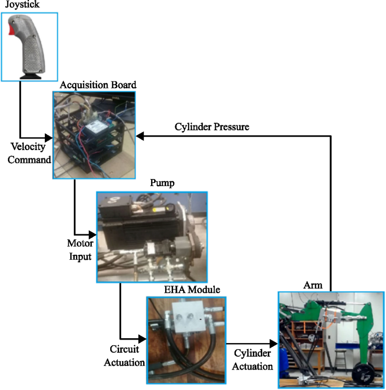
This study is built upon the novel energy-efficient EHA system designed by Costa and Sepehri [11]. Figure 1 illustrates the schematic of the hydraulic circuit. This system utilizes a bidirectional pump controlled by a servomotor to drive an asymmetric cylinder connected to a backhoe arm. The position of the cylinder rod is monitored using an incremental encoder, and the backhoe arm is subjected to varying loads, as shown in Fig. 1. The control input for this system is the voltage supplied to the servo motor governing the bidirectional pump. This pump directs flow to either side of the actuator based on the servomotor's operation, leading to pressure buildup. The pressure differential across the cylinder determines the exerted force. Pressure signals are crucial not only for controlling cylinder motion but also for condition monitoring, as is the focus of this paper. Therefore, denoising these pressure signals is also important for effective system control and health monitoring.
The data acquisition system for this EHA setup is built around a Raspberry Pi model 4 [12]. The test rig incorporates a mechanism to emulate internal leakage within the actuator chambers. This is achieved by regulating an orifice connecting both sides of the cylinder. Initially, the orifice is entirely closed, simulating a healthy (non-leaking) actuator. Subsequently, the orifice is opened progressively to represent varying degrees of leakage.
A dataset containing 48 signals was employed in this paper. These signals originated from the experimental EHA system and are categorized into two classes: healthy and faulty. The faulty signals exhibited various degrees of internal leakage within the actuator. These leakage levels are classified into three distinct categories: small (S), medium (M), and high (H). The objective of this study is to develop a method for discriminating between healthy and faulty actuator signals. Therefore, the three leakage levels within the faulty category were collectively considered as a single 'faulty' class for the classification task. The actuator was tested under three load conditions: no load (N), medium load (M), and high load (H). The experiments used both open-loop and closed-loop controls, using step and joystick inputs. For easy reference, each dataset has a unique five-letter code. The first letter (O or C) indicates open-loop or closed-loop control. The second letter (N, M, or H) represents the load level. The third letter (N, S, M, or H) shows the leakage level. Finally, the last two letters (Jo or St) signify joystick or step input (see Table 1). The dataset ONNSt is specifically plotted. This dataset represents the open-loop system with no load and no-leakage subjected to a step input for 50 seconds. Figures 2 and 3 illustrate the input, position, velocity, leakage, and pressure signals for the ONNSt and ONHSt datasets.
Table 1: Summary of abbreviation used for the datasets.
|
Operating condition |
Description |
Abbreviation |
|
System mode |
Closed-loop velocity control |
C |
|
Open-loop velocity control |
O |
|
|
Input mode |
Joystick input |
Jo |
|
Step input |
St |
|
|
Load mode |
No load |
N |
|
Medium load |
M |
|
|
High load |
H |
|
|
Leakage level |
No leakage |
N |
|
Small leakage |
S |
|
|
Medium leakage |
M |
|
|
High leakage |
H |
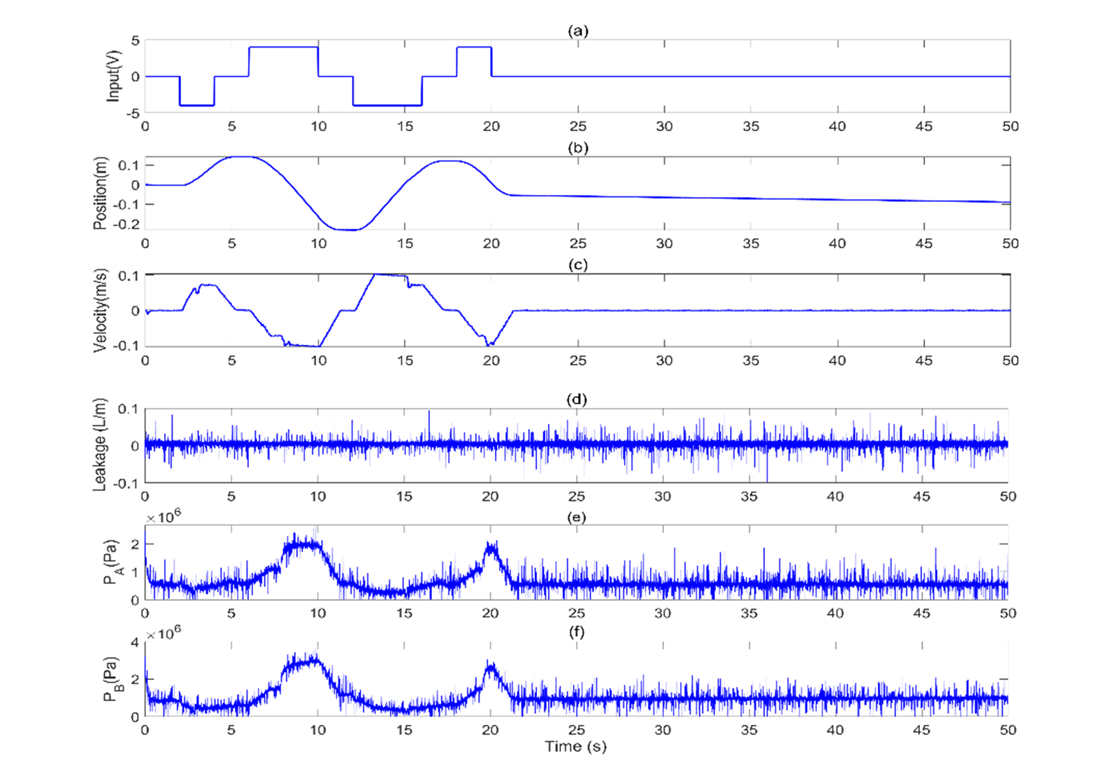
 ; (b) Position
  ; (c) Velocity,
  ; (d) Leakage level; (e) Measured pressure,
  ; (f) Measured pressure,
  .
.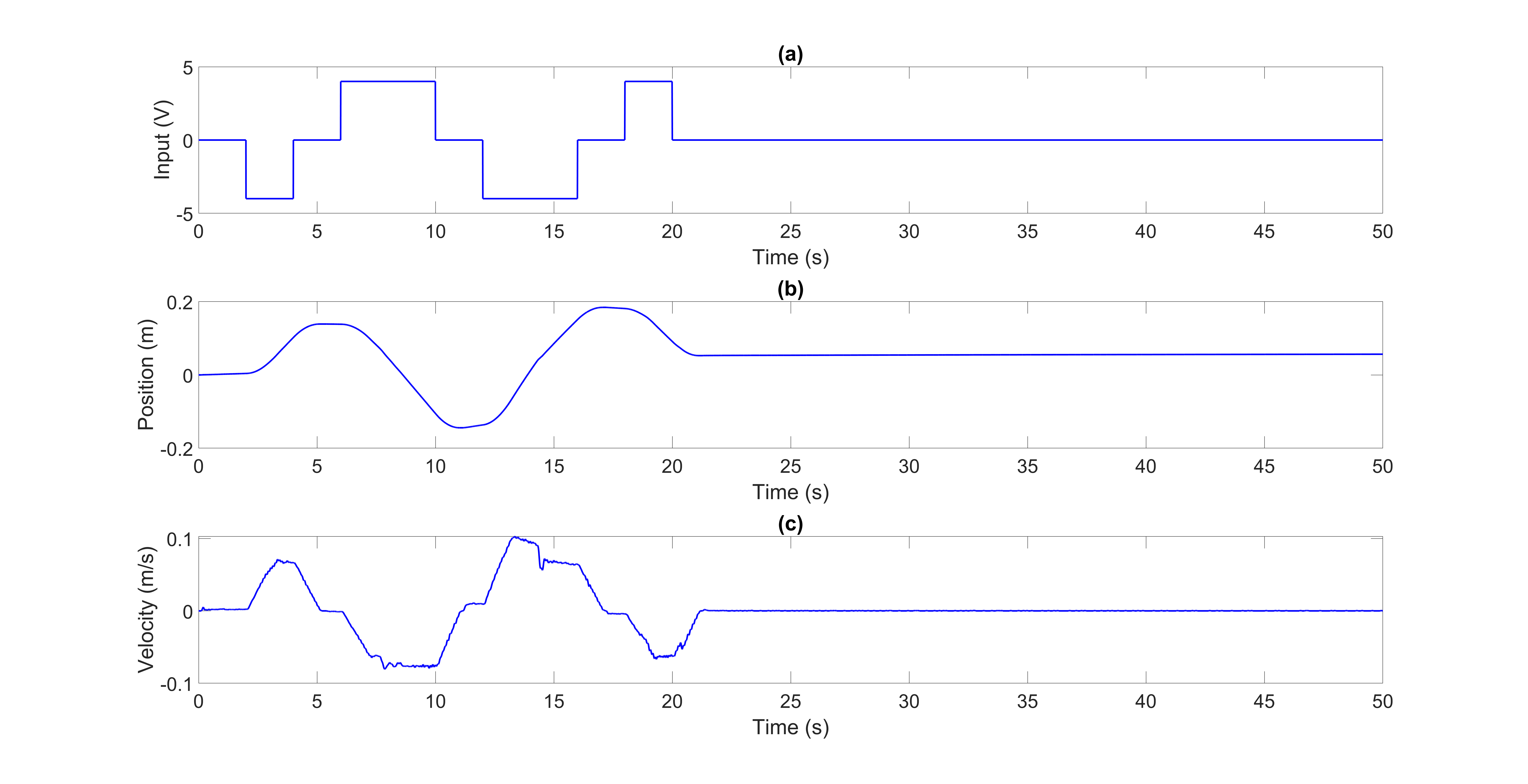
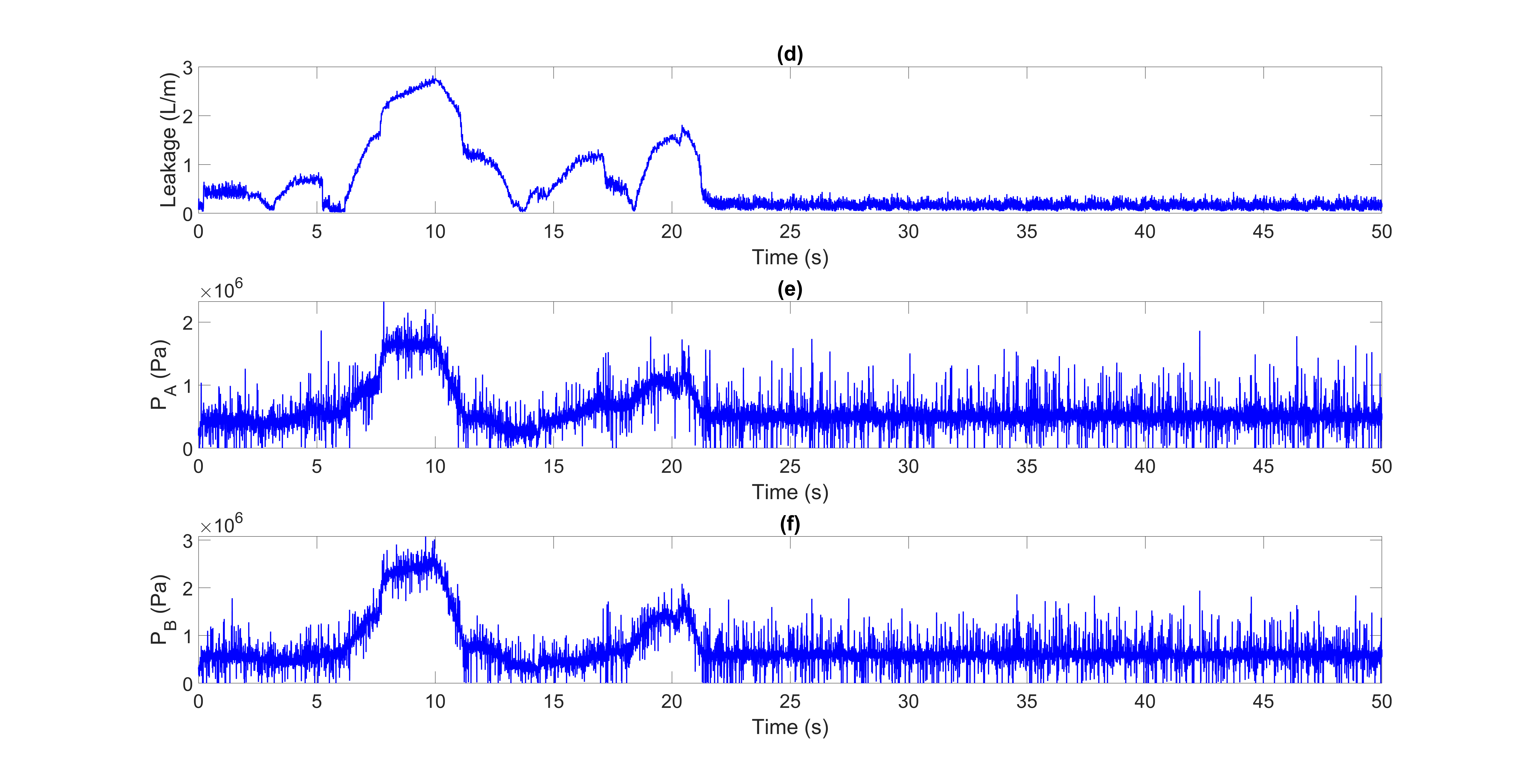
 ; (b) Position
  ; (c) Velocity,
  ; (d) Leakage level; (e) Measured pressure,
  ; (f) Measured pressure,
  .
.To apply our feature extraction method, it is necessary to first denoise the pressure signals. For this, we used the commonly used first-order low-pass filter (LPF) here [31]

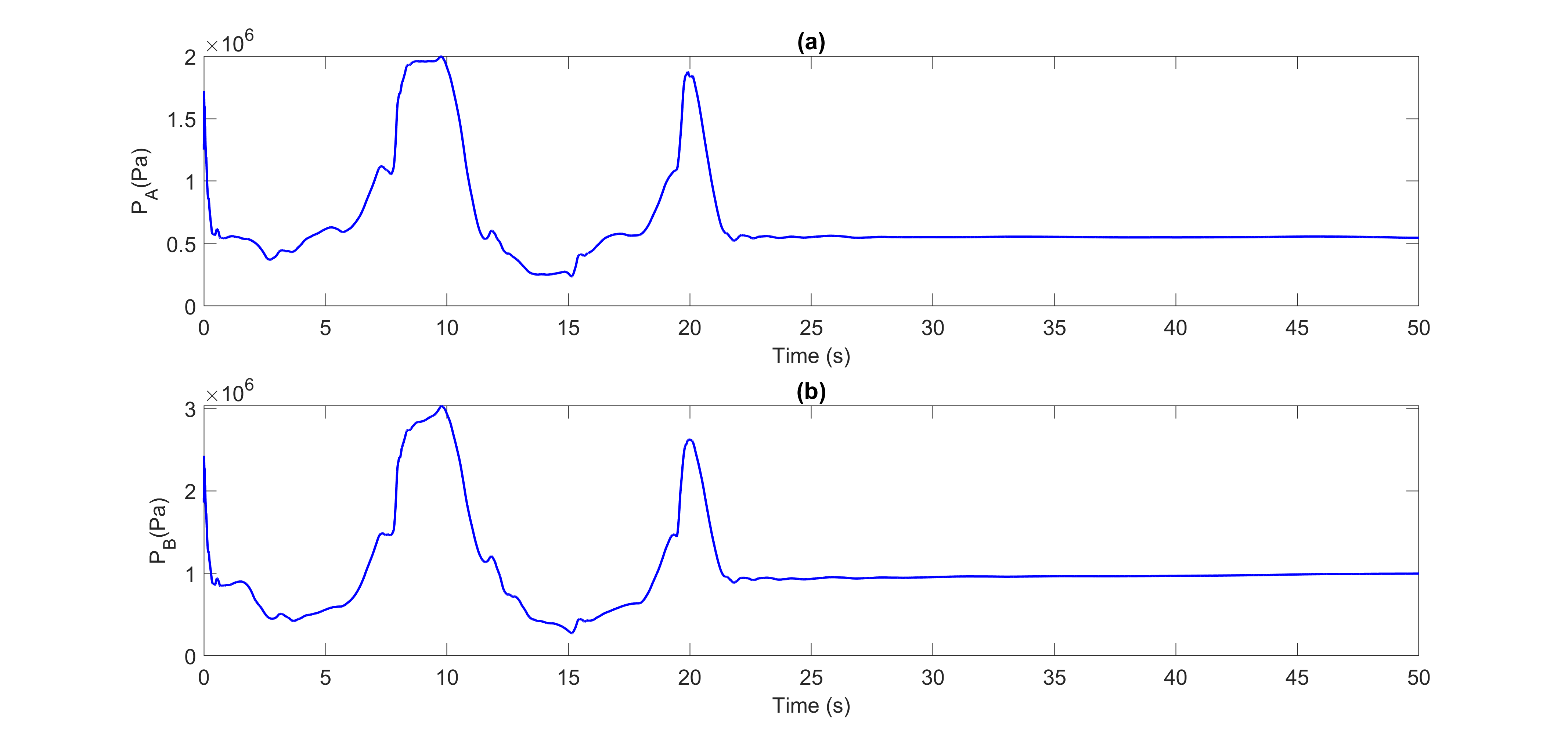
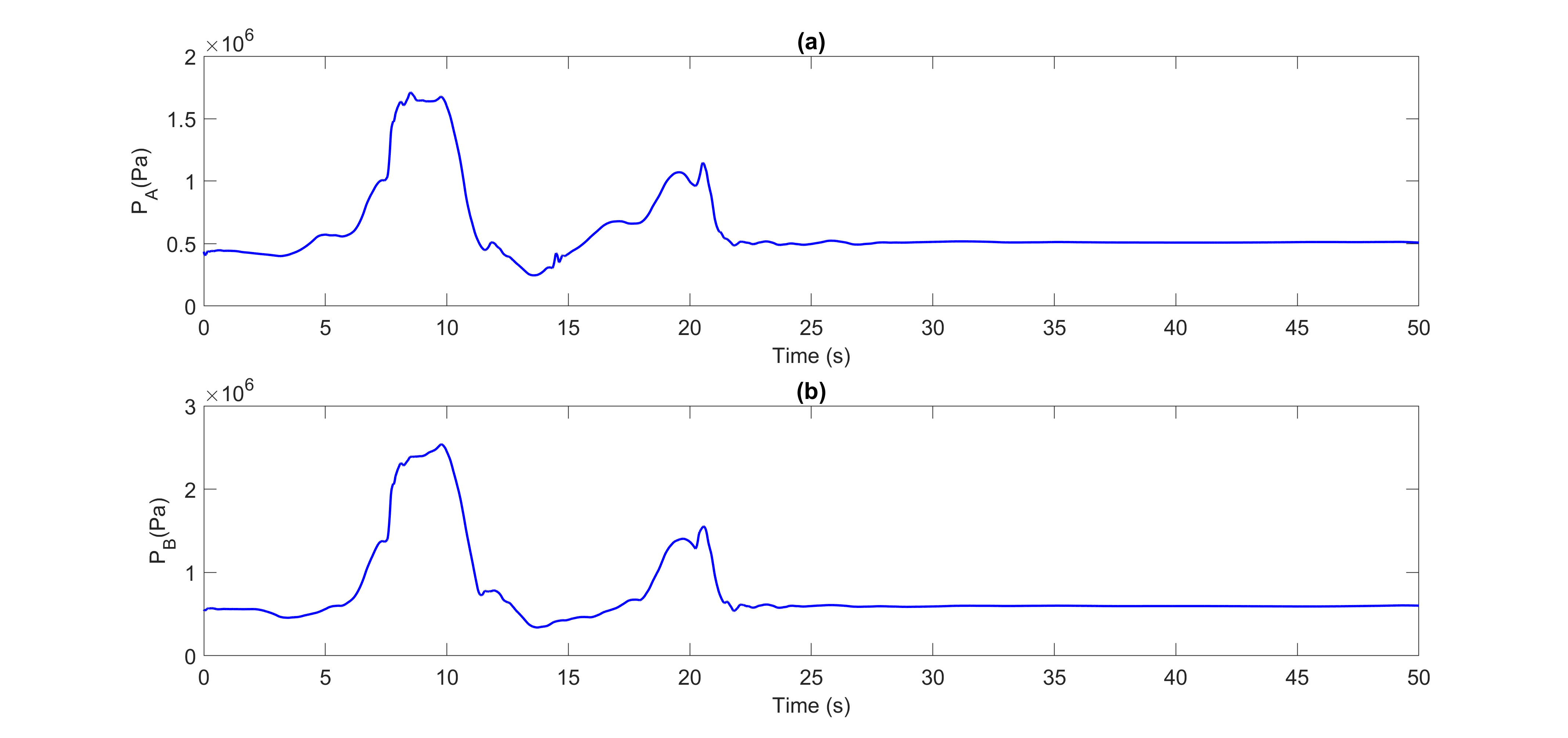
Using the LPF method, we denoised the pressure signals PA and PB. Figures 4 and 5 show the denoised pressure signals PA and PB for the datasets ONNSt and ONHSt.
3. Fractal Complexity Measure
Relevant features from the collected data are extracted and employed in an ANN for fault detection. The variance fractal dimension (VFD) method is utilized to extract features suitable for fault detection in the actuator signals. The VFD method is a well-established tool for analyzing complex time series, particularly those exhibiting self-affine properties [8]. Notably, self-affine time series display a characteristic power-law relationship between their variance and time increments as follows [8]

where y(∙) is a discrete sample of a time series sampled at time t. Taking the logarithm of both sides of equations and simplifying, the Hurst exponent (H) can be derived as follows

The Hurst exponent allows for the evaluation of the VFD through the following expression

for a time series with a single independent variable, H∈[0,1], E=1, and Dσ∈[1,2].
Unlike traditional monoscale analysis, polyscale analysis examines the signal across various scales simultaneously, utilizing volume elements (referred to as "vels"). To initiate the analysis, we first define the vels. We employ a mixed-size selection strategy as follows

where ⌊•⌋, is the floor function. The above 35 vel sizes is considered to obtain the VFD. We compute the variance of each subsequence, Vk,m, for the corresponding vel size nk in Eq. (5) as

where m=1,2,⋯,nk∈ N and Jk is the number of vels of size nk in the subsequences of differences and is defined as

where NE represents the number of samples in the entire extracted signals. If we take the average of the subsequences as

for each scale nk, we have the pairs (log2 (nk),log2 (Vk,ave)). To obtain the VFD, we use a robust linear regression technique called iteratively reweighted least squares (IRLS) [13] for line fitting

where s△ denotes the slope of the line. Accurate calculation of the VFD necessitates careful data pre-processing. This includes removing outliers and saturation points from the log-log plot values. Techniques like IRLS can be employed to mitigate the influence of outliers and improve the robustness of the VFD calculation.
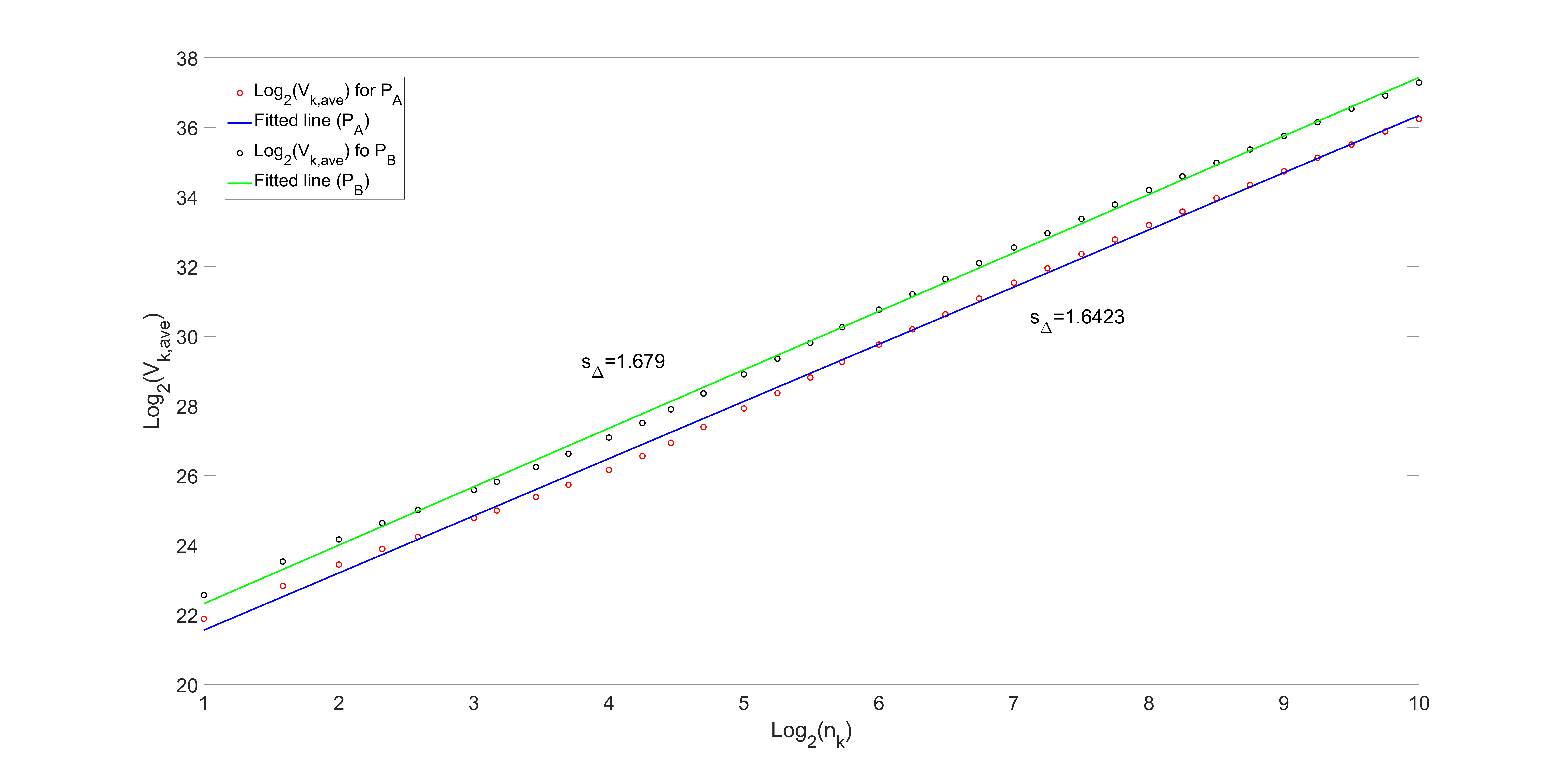
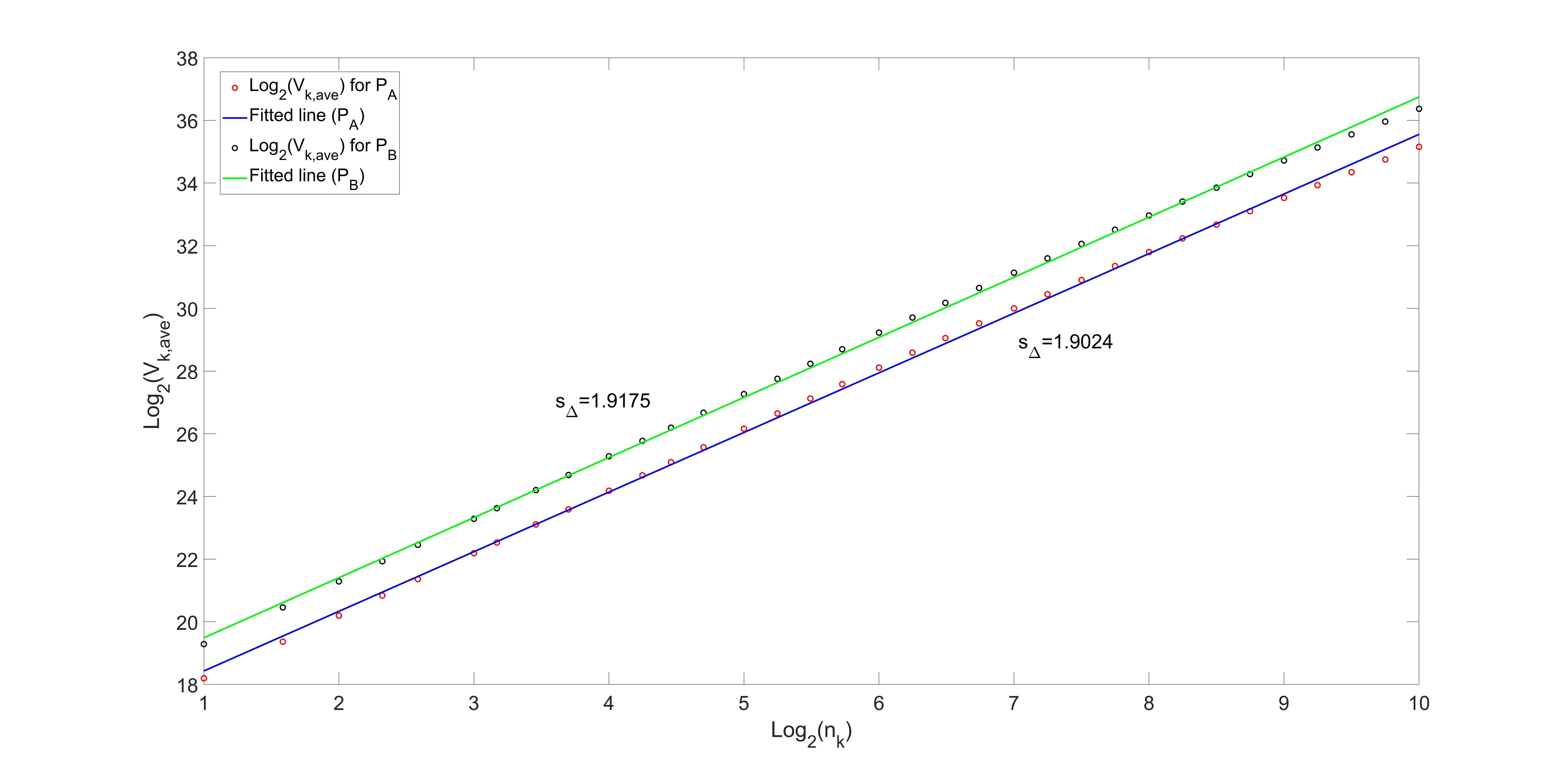
Figures 6 and 7 show the log-log plot of Vk,ave versus nk for datasets ONNSt and ONHSt, along with the corresponding fitted lines for pressures PA and PB. As can be seen, the data points form a linear relationship. It allows us to calculate the slope of the fitted lines. If they did not exhibit this linear behavior, the proposed feature extraction method would not be suitable for use in our classification method.
4. Neural Network Architecture
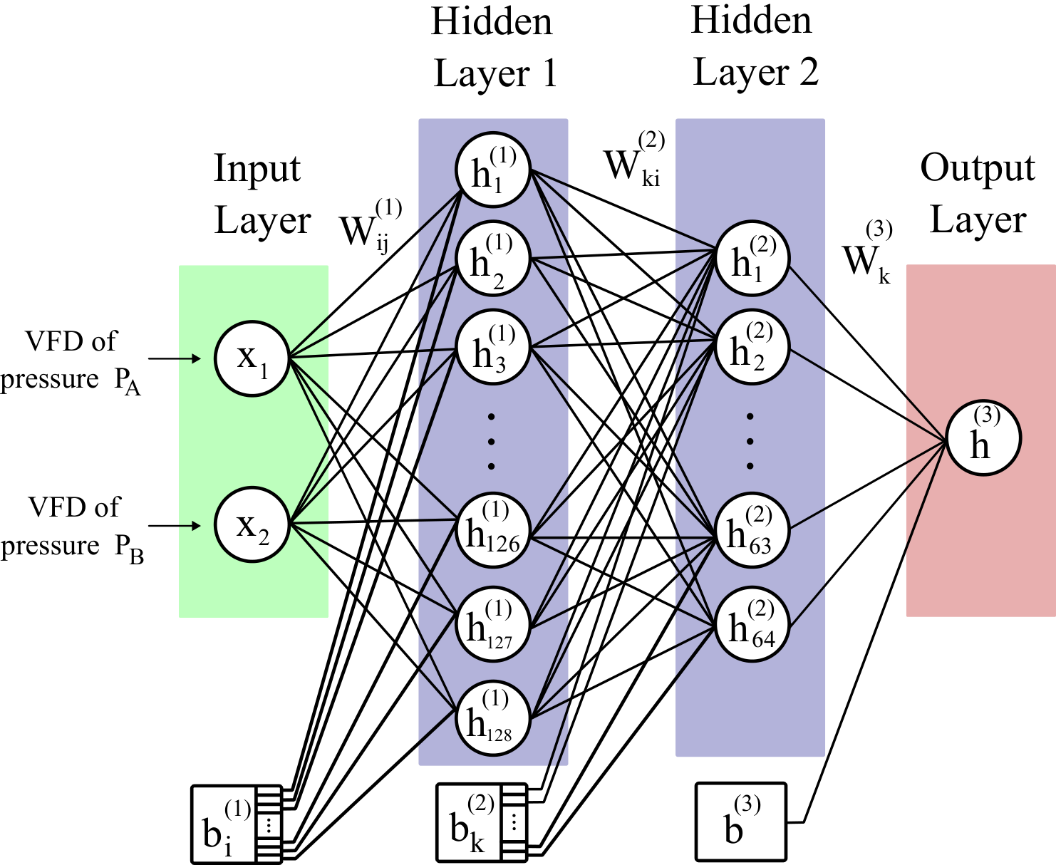
The proposed ANN for the fault classification of the EHA accepts two inputs as features extracted from the EHA, which are pre-processed and normalized for optimal neural network performance. The output layer provides a probability over 2 classes, indicating the probability of each class being the correct classification of the input. Training is conducted over 50 epochs with a validation split of 20% used to monitor and prevent overtraining on the training dataset. Datasets can be summarized as

where y(i) represents the label for sample i, where i=1,2,…,M, and M is the number of samples. x1(i) and x2(i) are the two extracted features from pressure signals PA and PB, respectively. The dataset is labelled based on the third letter of each file’s name, mapping to one of the two classes: healthy and faulty signals. We only use the no-leakage and small leakage datasets for our training and test the neural network on the rest of the datasets.
A stochastic gradient descent (SGD) optimization method is applied for optimizing the loss function in the ANN [14]. Instead of computing the gradient of the loss function over the whole dataset, SGD estimates the gradient based on a subset of the data, known as a minibatch. This makes SGD much faster for large datasets. Smaller batch sizes result in noisier gradients because they are based on less data. Therefore, the choice of appropriate batch size affects computational efficiency. Larger batch sizes can lead to faster convergence in terms of epochs because the gradient estimates are less noisy and more representative of the entire data set. However, it might require more computational resources per epoch. The binary cross-entropy is also used as the loss function, which can be defined as

where y represents the true label of the signal, indicating its health status. Here, 0 signifies a healthy signal, while 1 denotes a faulty one. p is the predicted probability of the class with label 1, as output by the model, and log is the natural logarithm.
4.1. Structure of the Layers
Figure 8 shows the structure of the neural network. Each neuron in the first layer computes a weighted sum of the inputs plus a bias and then applies an activation function. For neuron i in the first hidden layer, the output hi(1) is

where ![]() is the weight from input
is the weight from input ![]() to neuron
to neuron ![]() in layer 1,
in layer 1, ![]() is the
is the ![]() th input
feature,
th input
feature, ![]() is the bias for neuron
is the bias for neuron ![]() in layer 1,
and
in layer 1,
and ![]() is the
activation function. Similar to layer 1, each neuron in the second layer
computes a weighted sum of the outputs from the previous layer, adds a bias,
and then applies the activation function. For neuron
is the
activation function. Similar to layer 1, each neuron in the second layer
computes a weighted sum of the outputs from the previous layer, adds a bias,
and then applies the activation function. For neuron ![]() in this layer,
the output
in this layer,
the output ![]() is
is

where ![]() is the weight from neuron
is the weight from neuron ![]() in layer 1 to
neuron
in layer 1 to
neuron ![]() in layer 2,
in layer 2, ![]() is the output of neuron
is the output of neuron ![]() in layer 1,
in layer 1, ![]() is the bias for neuron
is the bias for neuron ![]() in layer 2,
and
in layer 2,
and ![]() is the activation function. For the neuron in the
output layer, the output
is the activation function. For the neuron in the
output layer, the output ![]() is
is

where  is the weight from neuron
  in layer 2 to
the single neuron in the last layer,
  is the output of neuron
  in layer 2,
  is the bias for the single neuron in layer 3, and
 is sigmoid
function.
4.2. Bayesian Optimization
Bayesian optimization is an important method for tuning hyperparameters in machine learning models [15]. In the context of the neural network, Bayesian optimization operates by constructing a probabilistic model, typically a Gaussian process (GP), to estimate the function and then iteratively selects the next set of hyperparameters based on an acquisition function that balances exploration (sampling where the model is uncertain) and exploitation (sampling where the model predicts high performance). The Bayesian optimization algorithm is as follow:
1. Input:
- Initial dataset {(𝑥𝑖,𝑦𝑖=𝑓(𝑥𝑖))}𝑖=1:𝑡
- Acquisition function 𝑢(𝑥)
- GP model for 𝑓(𝑥)
- For t=1:T do:
2.1. Model update:
- Update the GP model using all available data {(xi,yi=f(xi))}i=1:t.
- The GP posterior provides the mean μGP(x) and variance σGP(x)2 for any x, representing the predicted function values and uncertainty, respectively.
2.2 Optimize Acquisition Function:
- Use the GP posterior to define the acquisition function u(x).
- Solve the next point to evaluate by maximizing the acquisition function:

2.3 Evaluate Objective:
- Query the true objective f function at xt+1 to obtain the new observation yt+1 = f(xt+1).
2.4 Update Dataset:
- Append the new data point (xt+1,yt+1) to the dataset.
- Repeat the above steps until the max iteration is reached and return the point:

Bayesian optimization was used here to define a hyperparameter search space that considers three key parameters: learning rate, batch size, and activation functions in hidden layers. The learning rate, a critical factor in the convergence and performance of the training process, was varied within a range from 0.01 to 0.1. The batch size, dictating the number of samples processed before the model is updated, was considered within an integer range from 2 to 18. Finally, the type of activation function used in the hidden layers was also optimized, with options including; rectified linear unit (ReLU), hyperbolic tangent, and sigmoid activation functions. We employed gp_minimize from the skopt library in Python for Bayesian optimization. A maximum of 50 evaluations of the objective function is set to balance the exploration of the hyperparameter space with computational efficiency. Using Bayesian optimization, we successfully identified the most effective hyperparameters for our neural network model. The optimal learning rate was η=0.0862. The batch size was optimized to 12. Furthermore, the activation function was established as ReLU. A five-fold cross-validation was also employed on the dataset to show the model's performance. Table 2 reports the results from the Bayesian optimization process.
Table 2: Summary of weighted averaged results for 5-fold cross validation for Bayesian-optimized neural network.
|
Fold |
Accuracy |
Precision |
Recall |
F1-score |
|
Fold 1 |
93% |
93% |
93% |
93% |
|
Fold 2 |
93% |
93% |
93% |
93% |
|
Fold 3 |
97% |
98% |
97% |
97% |
|
Fold 4 |
97% |
98% |
97% |
97% |
|
Fold 5 |
93% |
100% |
93% |
96% |
|
Average |
94.6% |
96.4% |
94.6% |
95.2% |
To evaluate the performance of Bayesian optimization, the results are compared across four different cases. First, an ANN is considered without the application of Bayesian optimization for hyperparameter tuning. In this case, the learning rate is set to η=0.01, and the activation function in the hidden layer is ReLU. Additionally, three other classification methods are considered: support vector machine (SVM), random forest, and decision tree. A summary of the results is reported in Table 3. All classification algorithms have been implemented in Python.
Table 3: Summary of weighted averaged results from 5-fold cross-validation of common classification methods for fault detection.
|
Criteria |
ANN without Bayesian |
SVM |
Random forest |
Decision tree |
|
Accuracy |
91.6% |
93.2% |
92.4% |
84% |
|
Precision |
95.6% |
94% |
95.6% |
96.6% |
|
Recall |
91.6% |
93.2% |
92.4% |
84% |
|
F1-score |
93.2% |
93.4% |
93.4% |
88.2% |
5. Discussion of Results
This study introduced a novel fault detection model using Bayesian optimization within a neural network. The incorporation of Bayesian optimization allowed for fine-tuning of the ANN hyperparameters. It significantly enhanced the model's performance in classifying faults, as compared to traditional methods such as support vector machines, decision trees, and random forests. The superior performance of the Bayesian-optimized ANN can be due to its ability to optimize learning rate, activation functions in hidden layers, and batch sizes, which are critical in adapting to the hidden patterns of signal data from the EHA system.
The analysis also highlighted two particularly useful features for fault detection: the VFD of pressures in two sides of the hydraulic cylinder. These features were key in achieving high classification accuracy, proving cost-effective compared to other features such as velocity and position sensors. This finding is very important for practical applications, as it suggests a pathway toward fault detection with fewer sensors without sacrificing performance.
In this research, the exploration of hyperparameters was confined to learning rate, activation functions, and batch size. However, future studies could expand on this by considering other significant parameters such as the number of layers and the number of neurons in each layer, which might further enhance the model's accuracy, while reducing its complexity. Additionally, while the VFD proved to be an effective feature for fault detection, integrating additional features could potentially unveil more complex fault patterns and improve the performance of fault detection under varying operational conditions.
6. Conclusion
This paper discussed the application of Bayesian optimization within neural networks for fault detection of an electro-hydrostatic actuation system. More specifically, a feature extraction method based on variance fractal dimension was developed within the neural network. Features were extracted from either side of pressures in both the cap and rod sides of the hydraulic actuators. We employed Bayesian optimization for tuning hyperparameters. The proposed approach improved fault detection accuracy and outperformed conventional classification methods, such as Random Forest, SVM, and Decision Tree. The results indicated an average accuracy of 94.6%, precision of 96.4%, recall of 94.6%, and F1-score of 95.2% across 5-fold cross-validation. Further research will explore additional hyperparameters and integrate more features to classify different levels of fault, which can be more beneficial in industrial applications.
References
[1] Bradley Heinrichs, Nariman Sepehri, and A.B. Thornton-Trump, "Position-based Impedance Control of an Industrial Hydraulic," IEEE Control Systems Magazine, vol. 17, no. 1, pp. 46-52, 1997. DOI: 10.1109/37.569715. View Article
[2] Ali Maddahi, Nariman Sepehri, and Witold Kinsner, "Fractional-order Control of Hydraulically Powered Actuators: Controller Design and Experimental Validation," IEEE/ASME Transactions on Mechatronics, vol. 24, no. 2, pp. 796-807, 2019. DOI: 10.1109/TMECH.2019.2894105. View Article
[3] Hongjiang Cui, Ying Guan,Huayue Chen, and Wu Deng, "A Novel Advancing Signal Processing Method Based on Coupled Multi-Stable Stochastic Resonance for Fault Detection," Applied Science, vol. 11, no. 12, 2021. DOI: 10.3390/app11125385. View Article
[4] Jiyu Yan, Huijie Zhu, Xiaoqiang Yang, Youhui Cao, and Lifu Shao, "Research on Fault Diagnosis of Hydraulic Pump Using Convolutional Neural Network," Journal of Vibroengineering, vol. 18, no. 8, pp. 5141-5152, 2016. DOI: 10.21595/jve.2016.16956. View Article
[5] Ali Maddahi, Witold Kinsner, Nariman Sepehri, "Internal Leakage Detection in Electrohydrostatic Actuators Using Multiscale Analysis of Experimental Data," IEEE Transactions on Instrumentation and Measurement, vol. 65, no. 12, pp. 1-14, 2016, DOI: 10.1109/TIM.2016.2608446. View Article
[6] Lei Zhufeng, Qin Lvjun, Wu Xiaodong, Jin Wen, and Wang Caixia, "Research on Fault Diagnosis Method of Electro-Hydrostatic Actuator," Shock and Vibration, pp. 1-9, 2021. DOI: 10.1155/2021/6688420. View Article
[7] Kunpeng Zhu, Jerry Ying Hsi Fuh, Xin Lin, "Metal-Based Additive Manufacturing Condition Monitoring: A Review on Machine Learning Based Approaches," IEEE/ASME Transactions on Mechatronics, vol. 22, no. 1, pp. 509-520, 2017. DOI: 10.1109/TMECH.2016.2620987. View Article
[8] Witold Kinsner, "A Robust Variance Complexity Measure for Stochastic Self-affine Processes," in Proc. 18th IEEE International Conference on Cognitive Informatics & Cognitive Computing, ICCI*CC19, Polytechnic University of Milan, Milan, Italy; pp. 75-82, July 2019. DOI: 10.1109/ICCICC46617.2019.9146065. View Article
[9] Grzegorz Filo, "Artificial Intelligence Methods in Hydraulic System Design," Energies 2023, vol. 16, no. 8, DOI: 10.3390/en16083320. View Article
[10] Trevor Hastie, Robert Tibshirani, and Jerome Friedman, The Elements of Statistical Learning: Data Mining, Inference, and Prediction. Springer, 2009 (2nd ed.), 767 pages, {ISBN-13: 978-0387848570}.
[11] Gustavo Koury Costa and Nariman Sepehri, "Four-quadrant analysis and system design for single-rod hydrostatic actuators," Journal of Dynamic Systems, Measurement, and Control, vol. 141, no. 2, 021011 (15 pages), 2019. DOI: 10.1115/1.4041382. View Article
[12] Amirreza Mirbeygi Moghaddam, "Fault Detection and Fault-tolerant Control of Single-rod Electrohydrostatic Actuated System," M.Sc. Thesis. Winnipeg, Manitoba, Canada: University of Manitoba, Department of Mechanical Engineering, 2021, 135 pages. View Article
[13] Paul W. Holland and Roy.E. Welsch, "Robust Regression Using Iteratively Reweighted Least-squares," Communications in Statistics: Theory and Methods, vol. 6, no. 1, pp. 13-827, 1977. DOI: 10.1080/03610927708827533. View Article
[14] Quoc Tran-Dinh and Marten van Dijk, "Gradient Descent-Type Methods: Background and Simple Unified Convergence Analysis, " arXiv:2212.09413 [math.OC], (24 pages), 2022. DOI: 10.48550/arXiv.2212.09413. View Article
[15] Frank Hutter, Lars Kotthoff, and Joaquin Vanschoren, Automated Machine Learning: Methods, Systems, Challenges, Springer Cham, 2019, 223 pages, {ISBN-13: 978-3-030-05318-5}.

