Journal of Machine Intelligence and Data Science (JMIDS)

1. Introduction

As technology advances, systems modelling has become increasingly difficult. Furthermore, today’s complicated, high performing systems may contain more nonlinearities. As a result, traditional control methods, such as PID control, are often used at the cost of efficiency and performance. Modern Lyapunov-based controllers are more robust, which is important when stability is desired even with modelling assumptions and uncertainties. In many cases, however, the number of uncertainties makes using most Lyapunov-based controllers impractical. For example, a sliding mode controller used to control a system with high uncertainties would require a large controller gain, and, as a result, a high control output.

To feasibly control these systems, multiple globally robust controllers have been developed. These controllers generally use two methods to achieve stability no matter the uncertainty: limiting the form of the error in the system or estimating the maximum uncertainty. One example of the first method was given in [1]. The LQR-based controller was proven to cause stability so long as the uncertainties were in the image of the control influence matrix. On the other hand, the controller in [2] would result in stability issues when a certain parameter was larger than a linear combination of the uncertainty and its derivative. An estimator was created to keep the parameter above the linear combination. Both controllers were tested and performed adequately but are limited in their scope (linear systems for [1] and second-order SISO systems for [2]). These two controllers illustrate the need for a broadly applicable globally robust controller; such a controller would guarantee stability no matter the system form.

For under-actuated systems many different control methods have been developed using SMC. [3] compared four different types of SMCs used for underactuated systems. No estimation techniques are presented for tuning the parameters and chattering was also present causing issues in the real-time implementation of the designed controls strategies. [4] uses a combination of LQR and SMC wherein the states in the underactuated system are split within two different loops. While the proposed design is effective for the system defined, disturbance is present at various time intervals. Also, it might not work well in the presence of uncertainties or when the system model is not accurate. The concept introduced in [5] follows complex mathematical formulations which could result in challenges during practical implementation.

A controller with the potential to be broadly globally robust was introduced in [6] and developed in [7] and [8]. The controller method – known as Model Free Sliding Mode Control (MFSMC) – solved the issue of large uncertainties in the system by avoiding a system model entirely. Instead, it relied on the unity gain equation and assumptions which are as follows:

(1)

(2)

(3)

(4)

(5)

Where wherein n represents the system states, B is the control or input gain matrix and is given by B_ijϵR^n×m with m representing the number of inputs, is the control input and σ_u is the boundary constant in MFSMC. Sliding mode control techniques are then applied and the resultant controller is of the form:

(6)

(7)

Where is the sliding condition, is variable boundary layer discontinuous switching gain, β is the square root of B_ij,max/B_ij,min, I is the identity matrix, is discontinuous switching gain. A boundary layer was also introduced to reduce dithering. A derivation in a sliding mode context is given in [9].

These papers demonstrated MFSMC was applicable to all square systems (systems in which the number of control inputs is equal to the number of non-derivative states) so long as the bounds of the influence matrix were known. [10] proposed the use of an estimator for the parameter , which would avoid the need to know the bounds on the input matrix. Due to efficiency concerns, [11] adapted the estimator to find the matrix directly. While the controller-estimator combination stabilized several test systems, the performance of the estimator was sub-par in some circumstances.

Currently work is being performed to solve both limitations. In this work, both a method for estimating the bounds on the influence matrix and the use of a hyper-plane transformation for the control of non-square systems are presented. Results of using these techniques in a sliding mode context are presented. In the future, these methods will be adapted to MFSMC.

2. Sliding Mode Control

2.1. Boundary Estimation

Using a traditional estimator in MFSMC is more difficult than it may first seem – without a model, finding a suitable regression equation is not straightforward. The method in [11] was adapted using a least squares estimator with bounded gain forgetting. Rather than deriving the estimator from a relationship involving the influence matrix, [11] created a least-squares with bounded gain forgetting estimator using the sliding condition. The condition was developed as a part of sliding mode control:

(8)

(9)

Where Λ is positive definite matrix, is the difference between the current states and their desired values and “∘” is an element-wise product. When Eq. (8) is satisfied, the system is stable. The estimate is multiplied by a factor to estimate the matrix’s bounds. The new technique similarly uses the sliding condition. Given a system of the form:

(10)

the estimator’s goal is to find the influence matrix bounds. Start by substituting Eq. (10) into Eq. (9) and rearranging to obtain:

(11)

Next, multiply both sides by a factor which is 1 when the sliding condition is not satisfied and -1 in all other situations. Note doing so flips the inequality. The factor generalizes the inequality to all states of the sliding condition.

At this point, the derivation diverges for coupled and decoupled systems. First, consider the case when the system is decoupled (B is diagonal). If is a vector of the diagonal elements of B (B=diag(()), the left side reduces to:

(12)

The final step is to define the following values:

(13)

(14)

(15)

Using these definitions, the influence matrix bounds may be estimated as:

(16)

(17)

Where A⁺ is the pseudoinverse of A and B_k|kis the current bounds estimate. B_k|k-1 is the exact solution to the equation. However, if any of the current values of B are less than their corresponding maxima, some of the estimated values will be too low. For that reason, the actual estimate B_k|k is found by comparing the equation’s solution with the last estimates. A similar approach may be taken to derive an estimator for coupled systems. In testing, these definitions – which are derived from the maximizations of each side of the inequality – performed better than alternatives.

2.2. Hyper-plane Transformation

Using the MFSMC approach perfect tracking and stability for square MIMO systems have been obtained but additional methods are needed to guarantee tracking for underactuated (non-square) MIMO systems. A challenge in handling non-square systems is the non-invertibility of the input gain matrix, making the formulation of the control law impossible. A potential solution involves employing a coordinate transformation of the system. Through the transformation, the originally "non-square" matrix can effectively be "squared," overcoming the non-invertibility limitation and facilitating the formulation of the control law.

Consider the following system in the matrix form:

(18)

Where x represents the system states matrix, f represents the system functions in the matrix form, [B] is the non-square matrix and u is the control input matrix. A transformation matrix, [T] is considered for converting into the hyperplane, y:

(19)

Where the dimensions of matrix [T] = the dimensions of [B]^'. Eq. 19 can be rewritten as:

(20)

and the product of [[T][B]] is now square and invertible. The matrix [T] can be thought of as a weighing matrix. Since the system under consideration is underactuated, and states cannot display perfect tracking simultaneously, [T] can be used to track certain outputs "more heavily" than others.

By applying SMC for a varying boundary layer, the control law is given by Eq. (21):

(21)

Where is the best estimate of f. Now:

(22)

Where k^*(x) is the variable boundary layer discontinuous switching gain. k(x) is given by:

Moreover, the material balances are expressed by Equation (2). However, for each species i=1.2, the criterion of electrical neutrality is stated by Equation (3):

(23)

Where F(x) is:

(24)

The boundary layer equation is given by:

(25)

(26)

To apply the model-free SMC method to an underactuated MIMO system, knowledge of the size of the [B] matrix of the system is required to formulate the transformation matrix [T]. Once that is known, the model-free SMC scheme can be developed in the y coordinate system, in a similar manner to the derivation in square MIMO systems, and [T] is used to relate y to x, and vice versa.

3. Results

3.1. Simulation Results for Boundary Estimator in SMC

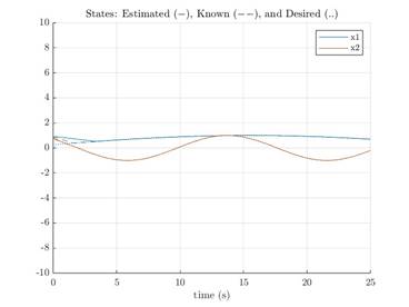
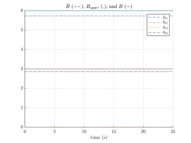
Simulation results for the nonlinear system represented by Eqs. (27) and (28) performed for SMC with and without boundary estimation are given in Figures 1 and 2.

(27)

(28)

Unsurprisingly, the controller with known bounds reaches the desired states faster overall (though state 2 of the estimated controller beats that of the regular SMC). The discrepancy is due to the time spent estimating the boundaries. Figure 2 shows the boundary estimates are above the maximum values. While the amount of estimation would seem to cause inefficiencies, Figure 3 indicates the estimated SMC has a lower control output.

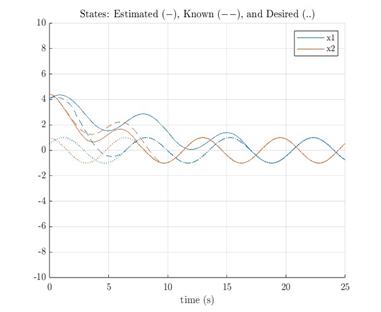
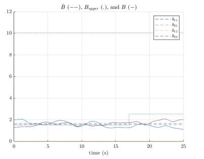
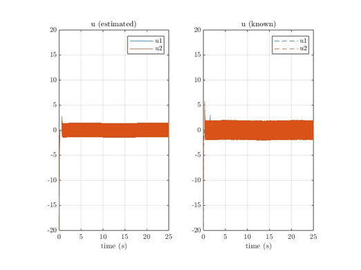
Figures 4 and 5 show the SMC with boundary estimation’s performance, this time against a coupled system. In Figure 5, the estimator is giving values of δ, a parameter related to B by:

(29)

The test system is the same as in Eqs. (27) and (28), except with b₁₂(t) and b₁₂(t) terms. Again, state 1 is sluggish, but the system is still stable.

3.2. Simulation Results for Hyper Plane Transformation in SMC

Simulation for traditional SMC with hyperplane transformation including boundary layer for the given system below was carried out in Simulink with fixed-step ode5 (Dormand-Prince) solver for 10 seconds.

(30)

(31)

The parameter values considered for the simulation are given in table 1.

Table 1 Parameters and their values used in the simulation

Parameters	Value
Bounds of a1	1 - 2
Bounds of a2	3 - 4
Transformation Matrix, [T]	[1 0.01]
Lambda, λ	20
Ita,	0.1
Phi,	0.1

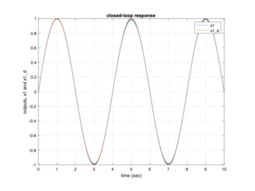
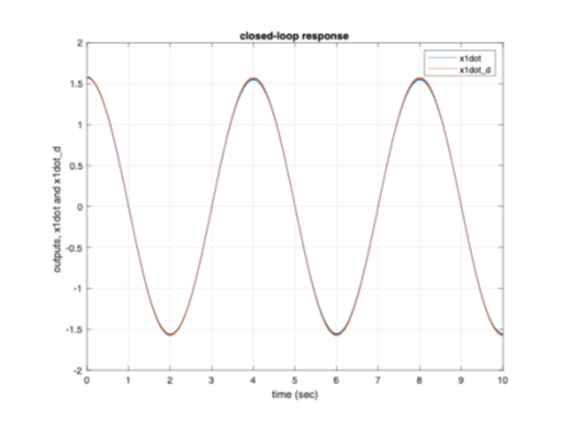
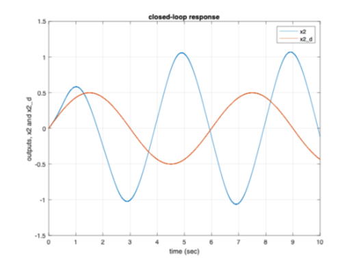
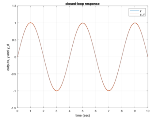
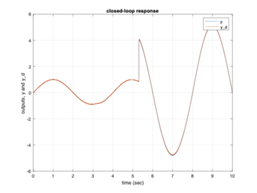
Figures 6(a and b) and 7(a and b) from the simulation result plots, represent the closed-loop responses of the states of the system (  ,   ,   , ) and the desired signals. There is close to perfect tracking for and with the desired signals but tracking of and is lacking. This is because of the values set in the transformation matrix, [T], and is more heavily tracked than and . Based on the requirement, [T] matrix can be set to either track and or and .

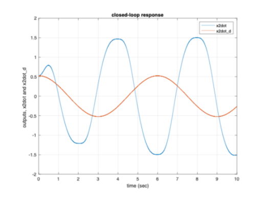
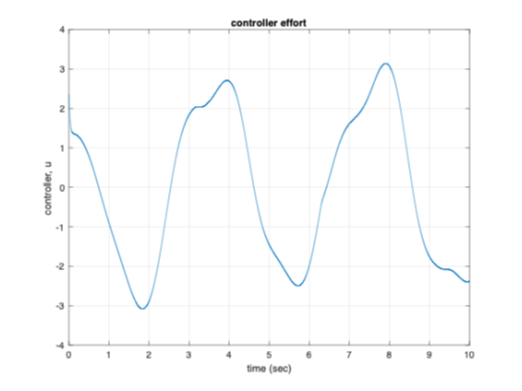
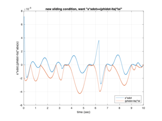
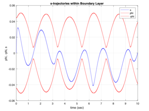
While the original signal tracking of the system is based on the [T] matrix, it can be seen from Figure 8a the transformed systems signal tracking is close to its desired value. The controller effort for the system is displayed in Figure 8b. Figure 9a shows that the system's sliding condition is satisfied which again proves the system is stable in the tracking sense. From Figure 9b, the S-trajectories lie within the defined boundary layer further proving the sliding condition is satisfied.

4.Conclusion

This paper introduced two methods: One, the integration of MFSMC approach with an online parameter (boundary) estimation method for complex nonlinear systems which allows for dynamic updates to the control law based on evolving system characteristics. The introduced approach includes a boundary layer to limit chattering and has precise tracking along with proven stability. The second method is the integration of hyperplane transformation with a traditional SMC for non-square MIMO systems with the inclusion of boundary layer. The tracking in this method depends on the values chosen in the transformation matrix. The next steps would be to apply both methods to model-free control and evaluate their performance. Upon obtaining the results for model-free control then this type of control approach can be applied to any physical systems making it more robust and stable.

References

[1] H.-P. Pang and G.-Y. Tang, “Global Robust Optimal Sliding Mode Control for a Class of Uncertain Linear Systems,” presented at the Chinese Control and Decision Conference, 2008, pp. 3509–3512. View Article
[2] Z. Huang and C. Sun, "Adaptive Global Robust Tracking Control for Uncertain Dynamic Systems," Int. J. Control Autom. Syst., vol. 21, no. 4, pp. 1070-1079, Apr. 2023. View Article
[3] S. Din, Q. Khan, F. Rehman, and R. Akmeliawanti, "A Comparative Experimental Study of Robust Sliding Mode Control Strategies for Underactuated Systems," IEEE Access, Vol. 5, pp. 10068-10080, 2017 View Article
[4] R E. I. Mohamed and A. Karaarslan," Stabilization of Quadcopter Using the Combination of LQR And SMC Methods," International Marmara Sciences Congress Proceedings Book, 2022
[5] B Lu, Y Fang and Ning Sun," Continuous Sliding Mode Control Strategy for a Class of Nonlinear Underactuated Systems," IEEE transactions on Automatic Control, vol. 63, no. 10, 2018 View Article
[6] A. Mizov, "A Model-Free Control Algorithm Derived Using the Sliding Model Control Method," Rochester Institute of Technology, 2015.
[7] R. M. Reis, "A New Model-Free Sliding Mode Control Method with Estimation of Control Input Error," Rochester Institute of Technology, 2016.
[8] F. El Tin, "A Model-Free Control System Based on the Sliding Mode Control Method with Applications to Multi-Input-Multi-Output Systems," Rochester Institute of Technology, 2017.
[9] J.-J. E. Slotine and W. Li, "Chapter 7: Sliding Control," in Applied Nonlinear Control, Prentice Hall, 1991, pp. 277-310. onal Conference on Design & Test of Integrated Micro & Nano-Systems, Sfax, Tunisia, 2021, pp. 1-6.
[10] M. S. Islam, "A Model-Free Control System Based on the Sliding Mode Control with Automatic Tuning Using as On-Line Parameter Estimation Approach," Rochester Institute of Technology, 2020.
[11] N. Hutson, "Model-Free Sliding Mode Control in the Lateral and Direction Dynamics of an Aircraft," Rochester Institute of Technology, 2023. View Article