Journal of Machine Intelligence and Data Science (JMIDS)

1. Introduction

In the realm of financial forecasting, predicting stock market indices continues to be a formidable challenge due to the inherent complexities, intricacies, and volatile nature of stock markets. Market movements are influenced by a myriad of factors, making the prediction task all the more difficult. The Efficient Market Hypothesis (EMH) [1] and the Random Walk Theory [2] postulates that stock prices are essentially unpredictable, suggesting that future prices are not necessarily dependent on past prices. The prediction task is further complicated by the dynamic nature of markets. According to [3], attempts to establish successful forecasting approaches rarely result in stable and enduring predictive patterns. This transience of profitable forecasting patterns underscores the difficulty of consistently achieving accurate predictions over extended periods. [4] suggests that even with the application of advanced AI strategies, such as machine learning algorithms for technical and fundamental analysis, the results have been median at best, implying that it may be premature to claim that AI technology can consistently beat the stock markets. Similar findings have been echoed in other research, further underscoring the formidable challenge of efficient stock market prediction. (see e.g., [5], [6]). Still, some research has indicated the possibility of prediction under certain circumstances, be it specific time frames, conditions, or with specific indices or stocks. (see e.g., [7]-[11]). These studies imply that the ability to predict markets could be context-specific. Recent advancements in computational power and the rise of machine learning algorithms have provided a fresh perspective on financial forecasting. Regression models, which predict a continuous outcome, have been particularly useful in this domain. Unlike classification models that predict discrete outcomes, regression models provide a more nuanced understanding of market trends by predicting specific prices or index values. Previous studies have delved into a range of time series decomposition methods aimed at forecasting stock market indices. Prominent among these methods is the Empirical Mode Decomposition (EMD) [12], and its subsequent variations like the Complete Ensemble Empirical Mode Decomposition with Adaptive Noise (CEEMDAN) [13]. Examples of applications in forecasting stock indices using these methods can be found in studies such as those by [14]-[16]. Alternatively, some researchers have employed the Seasonal-Trend decomposition using LOESS (STL) [17] for similar forecasting endeavors (see e.g., [18], [19]). Another notable approach is the Seasonal Decomposition by moving average, as discussed in [20], with practical applications illustrated by [21].

Given these advancements and challenges, we sought to explore an innovative approach. Building on prior research, our study uniquely combines various decomposition techniques for enhanced stock forecasting. Support Vector Regression (SVR) emerged as a superior method for forecasting the sub-waves generated through our decomposition techniques. The spectrum of models tested ranged from simpler non- recursive methods employing Seasonal Decomposition by moving averages, STL, or CEEMDAN to more intricate recursive ones.

Of particular note was a recursive model that first decomposed the stock index using CEEMDAN and subsequently decomposed each of those sub-waves with STL. This model stood out in our empirical analysis, showcasing the zenith of predictive accuracy. Intriguingly, models incorporating CEEMDAN consistently outperformed those using EMD, highlighting CEEMDAN's prominence in our tests.

Our models underwent meticulous comparison against one another and were benchmarked against seminal models from existing literature. This rigorous evaluation framework ensures a holistic assessment of our methodology, contextualizing its position in the broad landscape of stock index forecasting.

The remainder of this article is organized as follows:

In Section 2, the Literature Review, we delve into methodologies in stock index prediction that employ decomposition techniques or closely related methods, contextualizing our approach amidst established practices.

Section 3, Software and Data Sources, details the technological tools and datasets that drive our research.

Section 4, the Data Overview, presents the specifics of the datasets, laying the groundwork for our experimental discussions.

Section 5, our Methodology, we cover the entirety of our experimental approach, including the models we tested, the criteria we employed for comparison, our experimental setup, and our unique approach to feature engineering for SVR.

Section 6, Experiment and Results, presents the outcomes of our research in detail, comparing the various methodologies we employed, and analyzing the resultant insights, all supported by a chart comparing the performance of the best model found to actual data.

Lastly, in Section 7, the Conclusion and Future Work, we sum up our findings and provide avenues for subsequent research endeavors.

2. Literature Review

The forecasting landscape of stocks and stock-indices has witnessed the application of a myriad of methods ranging from statistical models to advanced machine learning techniques. Yet, decomposition stands out as a powerful mechanism to uncover intricate patterns within stock market data. This review predominantly centers on decomposition methodologies, providing a prelude to more advanced and hybrid techniques used in forecasting. Decomposition has long been a foundational tool in time series analysis. Its primary objective is to parse a series into distinct components, usually trend, seasonality, and residual, thereby simplifying the forecasting process.

One of the prominent methods in the domain of time series decomposition is the Empirical Mode Decomposition (EMD) [12]. At its core, EMD facilitates the decomposition of a time series into a set of oscillatory components known as intrinsic mode functions (IMFs). Unlike traditional decomposition techniques that rely on a priori basis functions, EMD dynamically adapts to the inherent oscillations in the data. The technique identifies the highest and lowest points in a time series and computes the mean envelope by averaging the upper and lower envelopes obtained through cubic spline interpolation. The detail extracted from subtracting this mean from the data constitutes an IMF. This process is recursively applied until the residual becomes monotonic, resulting in a series of IMFs which capture cyclic behaviors across different time scales.

Building on the foundation set by EMD, the Complete Ensemble Empirical Mode Decomposition with Adaptive Noise (CEEMDAN) was proposed as an enhancement [13]. Recognizing the occasional challenge posed by noise in EMD, CEEMDAN introduces white noise to the data multiple times, decomposes each noisy version with EMD, and then averages the results, thus giving a more robust decomposition. This variant has been extensively explored in stock market forecasting. For instance, Jin et al. [14] integrated EMD with deep learning architectures, highlighting its efficacy in disentangling intricate patterns in stock data.

The Seasonal Decomposition of Time Series (STL) is another pivotal method in time series decomposition [17]. Unlike methods that impose a rigid structure on the time series, STL offers flexibility in capturing seasonality. The STL method decomposes a time series into three components: trend, seasonal, and remainder (or residual). It employs a sequence of "loess" (locally weighted scatterplot smoothing) methods to extract the trend and seasonal components. One of its notable strengths is its ability to handle any type of seasonality, not just the fixed periodic seasonality seen in some series. Due to its robustness and adaptability, STL has found applications in various fields, including stock market forecasting.

Yet another tool for time series decomposition is Seasonal Decomposition by moving averages (SDMA) [20]. This method, more traditional in nature, is built upon moving averages and is particularly effective for series with stable seasonality patterns. In SDMA, a time series is broken down into its trend-cycle, seasonal, and irregular components. The simplicity and computational efficiency of SDMA make it a popular choice, especially when the focus is more on trend and seasonality extraction rather than intricate pattern identification.

Several studies in the literature have harnessed these decomposition techniques in the context of stock market forecasting. Using the EMD technique previously discussed, Jin et al. [14] broke down complex stock price sequences into simpler sequences for easier forecasting. They then extracted investors' sentiments by analyzing comments from stockholders on StockTwits and Yahoo Finance using a modified CNN. The EMD-processed data, combined with this sentiment analysis, was input into an enhanced LSTM model with attention, leading to superior prediction accuracy on AAPL data. Rezaei et al. [15] decomposed financial time series of major stock indices like S&P500 and Dow Jones into multiple intrinsic mode functions (IMFs) and residuals. Each IMF and residual was individually subjected to analysis using neural networks to unveil hidden price trends and relationships. The predictions from each component were then aggregated to offer a comprehensive forecast for the whole index. In another study, Lv et al. [16] used CEEMDAN to decompose indices like the S&P500 and DAX into Intrinsic Mode Functions (IMFs). Stationary sequences of these IMFs were analyzed using ARMA, while non-stationary sequences utilized LSTM models. The combined results from both methods yielded superior prediction accuracy over seven other benchmark models when tested on various global stock indices. [18] employed machine learning to forecast the Nikkei 225 stock index over a five-day period. Four daily stock-price indicators (SMA, WMA, EMA, SG) were decomposed into trend and seasonal components using STL. These decomposed elements served as inputs for a multivariate two-way LSTM model. The model executed both regression (forecasting actual prices) and classification (anticipating price direction), achieving accuracy in predicting price direction at 66.25%. Another study that utilized STL was conducted by He et el. [19]. In their approach, financial data was decomposed into seasonality, trend, and residual components. The seasonal component, consistent across financial markets, was retained based on a 12-month cycle. The trend was captured using a cubic polynomial fit. For the residual component, reflecting post-decomposition irregularities, they employed a Dendritic Neuron Model, which is an ANN with a structure inspired by biological neural architectures. This methodology, tested on 16 real-world stock market indices, showcased superior accuracy compared to other conventional models. Another notable approach to data decomposition is presented by [21]. In their study, a prediction method leveraging a form of seasonal decomposition, named SABL was introduced. This method predominantly utilizes Binary segmentation and Local polynomial regression techniques. The approach emphasizes the benefits of decomposing a series into its trend, seasonal, and residual components to enhance forecasting. While particularly effective for stock prices, its application to other assets, such as exchange rates, requires careful consideration. Building upon the foundational work highlighted in the preceding studies, our research carves out a unique niche. Our study distinguishes itself through its innovative use of recursive decomposition in financial forecasting. While decomposition is a recognized approach, our recursive method delves deeper into the inherent structures of financial data, uncovering patterns often overlooked by traditional techniques. Coupled with a contemporary prediction model, our methodology provides a comprehensive analysis of financial patterns, and its adaptability promises applicability across various financial assets.

3. Software and data sources

The research utilized Python 3.9.7 in conjunction with the Spyder 5.1.5 IDE. Regression analyses were performed using the various algorithms available in the sklearn package [22]. Data for this research was sourced from Yahoo Finance [23] via the Python package yfinance [24]. Evaluation of regression results employed the sklearn.metrics Python package [25].

4. Data Overview

The study utilizes daily closing prices of three major stock indices: NASDAQ 100, Dow Jones, and DAX. Data was sourced from January 1, 2010, to September 15, 2022. This timeframe encompasses 3198 trading days for the NASDAQ 100 and the Dow Jones, while the DAX spans 3222 trading days.

A chronological train-test split was adopted: the initial 2848 trading days were allocated for training for the NASDAQ 100 and the Dow Jones, from January 1, 2010, to April 27, 2021. For the DAX, the first 2872 trading days were used for training, spanning from January 1, 2010, to May 6, 2021.

The subsequent 350 trading days, starting from April 28, 2021, for the NASDAQ 100 and the Dow Jones, and from May 7, 2021, for the DAX, up to September 15, 2022, were designated for testing. This represents roughly 11% of the entire dataset for all three indices.

5. Methodology

5. 1. Models Tested

We evaluated a diverse set of prediction models, encompassing both traditional and recursion-based decomposition techniques. To succinctly recap:

• Simple Moving Average Decomposition (SMA): A non-recursive model employing Seasonal Decomposition using moving averages.
• CEEMDAN Model (C): A non-recursive model exclusively utilizing CEEMDAN.
• STL Model (STL): A non-recursive model leveraging STL Decomposition.
• SMA-STL Recursive Model (SMA-STL): A recursive model initiating with SMA Decomposition of the primary stock index, with each resulting sub-component further undergoing STL Decomposition.
• CEEMDAN-SMA Recursive Model (C-SMA): A recursive model beginning with CEEMDAN Decomposition, followed by SMA Decomposition of each resultant CEEMDAN sub-wave.
• CEEMDAN-STL Recursive Model (C-STL): A recursive model initiating with CEEMDAN Decomposition, succeeded by STL Decomposition of each resultant CEEMDAN sub-wave.
• STL-CEEMDAN Recursive Model (STL-C): A recursive model beginning with STL Decomposition of the primary stock index, with each resultant sub-component further decomposed using CEEMDAN.

For every model, our aim was to predict the succeeding value of each component, specifically a one-day-ahead forecast. Through comprehensive testing, Support Vector Regression (SVR) emerged as the consistently superior predictor across all models.

To provide further clarity on our modeling approach, we detail the specific parameters used for each technique: For the SMA, we adopted the configuration: 'model=additive`, 'two_sided=False`, and 'extrapolate_trend=freq`. In the CEEMDAN model, ensuring consistent noise generation was crucial, so we set the noise seed using 'ceemdan.noise_seed(1234)`. For the STL decomposition, the seasonal component was specified as 'seasonal=5`.

Detailed performances and comparisons will be elaborated upon in the subsequent sections.

5. 2. Comparison Criteria

The predictive performance of our models is assessed using a combination of widely recognized metrics and a metric introduced in this study, the Average of Absolute Return from Value to Value (AARV). The metrics utilized are:

• AARV (Average of Absolute Return from Value to Value): This metric offers a more intuitive understanding of daily fluctuations, providing insight into the average magnitude of changes between consecutive data points. It's defined as:

(1)

where p_i is the price at point i, and N represents the total number of data points in the series.

• RMSE (Root Mean Square Error)
• MSE (Mean Square Error)
• MAPE (Mean Absolute Percentage Error)

For all metrics except AARV, their standard definitions as implemented in the sklearn.metrics Python package were used, as referenced in the Software and Data Sources section.

5. 3. Experimental Setup

We tested the predictive accuracy of various models using one-step-ahead prediction for the three indices previously mentioned. For each model, every final sub-component was individually predicted for the subsequent day. The aggregate of these predictions yielded the forecasted value of the original index. The rationale for this method is that predicting each sub-component, being a simpler waveform with more discernible patterns, is ostensibly more accurate and feasible than forecasting the original index directly.

5. 4. Feature Engineering for SVR

Upon comparing various machine learning methods for predicting the next value of each sub-component, Support Vector Regression (SVR) emerged as the optimal choice for all sub-component types. Specifically, we utilized the linear kernel parameter for SVR. The default parameters provided by the sklearn.svm.SVR [26] implementation were primarily used, with some modifications based on our experimentation.

Deep analysis revealed that the predictive approach for the sub-wave obtained at the final stage of decomposition, when derived from SMA or STL, depended on the type of the sub-component.

• Trend sub-component: The most accurate predictions were obtained using the last 20 values as input features to the SVR. This aligns with the nature of the trend, which is often a smooth progression without abrupt deviations. The intuition here is that recent values can predict the immediate future due to the trend's consistent nature. For preprocessing, we first applied differentiation to represent day-to-day changes. The differentiation is given by:
  

  (2)
  
  where Δy_t represents the day-to-day change in the trend sub-component value at time t, y_t is the trend sub-component value at time t, and y_t-1 is the trend sub-component value at the previous day, t-1. Following this differentiation, we applied the MinMaxScaler transformation. Both transformations were applied to the training data, and post-prediction values were reverse-transformed to the original scale. The use of differentiation emphasizes local changes, and normalization ensures SVR operates optimally since it's sensitive to feature scales.
• Seasonality and Residual sub-components: For the seasonality component, given its nature which captures repeating patterns over fixed periods, it is inherently stationary. As such, differentiation wasn't deemed necessary. Meanwhile, the residuals, which represent the irregularities or noise after extracting other patterns from both STL and SMA, appeared to be relatively stationary upon examination. Consequently, differentiation wasn't applied to them either. For both sub-components, we directly applied the MinMaxScaler normalization to the original values. The subsequent processing and prediction methodology for these sub- components mirrored that of the trend sub- component.

Conversely, for intrinsic mode functions (IMFs) obtained from CEEMDAN during the final decomposition stage, the best predictions were obtained using merely the last 5 values for each IMF. The residue (or the trend component from CEEMDAN) was treated similarly. Data transformation was consistent with the process described earlier, applying differentiation followed by MinMaxScaler normalization.

Table 1 summarize the different procedures adopted for creating the input features to best predict each sub-component type.

Table 1. Summary of procedures for creating input features.

Sub-Component	Input Features (Last Values)	Transformations
Trend (SMA/STL)	20	Differentiation + MinMaxScaler
Seasonality/Residual (SMA/STL)	20	MinMaxScaler
All (CEEMDAN)	5	Differentiation + MinMaxScaler

6. Experiment and Results

In this section, we outline the results of our forecasting experiments conducted on three prominent stock indices: Nasdaq 100, Dow, and Dax. The primary objective is to discern which forecasting methodology—recursive or non-recursive—offers superior predictive capabilities for stock movements based on our selected metrics MAPE, RMSE, and AARV.

Evaluating the MAPE in conjunction with the AARV provides invaluable insights into the real-world predictive accuracy of our models. By contrasting the MAPE's error percentage with the average rate of stock value fluctuations (AARV), we can better assess the relative significance of prediction errors in the backdrop of standard market volatilities. For instance, a MAPE value lower than the corresponding AARV for an index indicates that our model's predictions surpass the average market volatility. This is significant as it implies that our model is capable of making accurate predictions that are not just reflective of general market fluctuations, but are indicative of a deeper, more nuanced understanding of market dynamics.

All models exhibited R² values of 0.94 and above, indicating a high degree of fit. We prioritized RMSE and MAPE for a more direct assessment of predictive accuracy. These metrics showed that both the recursive and non-recursive models achieved commendable accuracy across all indices, with the recursive models, particularly the C-STL approach, demonstrating superior performance. The C-STL model, for instance, achieved a MAPE score of 0.25% for the Dow index, significantly lower than the AARV of 0.77%, highlighting its exceptional predictive capability.

The standout performance of the C-STL model can be attributed to its hybrid approach, combining the strengths of both CEEMDAN and STL decomposition. The STL model's effectiveness, even when used independently, is evident from our results. By initially deploying CEEMDAN, we decompose the data into 8 or 9 simpler sub-components, allowing the STL method to then focus on these less complex segments. This step enhances the STL's ability to identify more nuanced patterns and trends, contributing to the superior performance of the C-STL model. The combination of CEEMDAN's noise reduction with the STL's robust seasonal decomposition facilitates a more detailed and accurate analysis of market dynamics, as demonstrated by our experimental data.

Table 2 presents the findings from our non-recursive models, while Table 3 does the same for the recursive counterparts.

Table 2. Performance of Non-Recursive Models.

	Nasdaq 100			Dow			Dax
AARV	1.23%			0.77%			0.93%
Model	RMSE	MSE	MAPE	RMSE	MSE	MAPE	RMSE	MSE	MAPE
SMA	233.7	54,609.7	1.29%	371.3	137,843.4	0.85%	192.3	36,983.7	0.99%
C	128.1	16,407.3	0.72%	222.4	49,460.3	0.52%	104.9	11,011.3	0.55%
STL	92.3	8,523.2	0.50%	153.5	23,567.2	0.35%	73.5	5,409.4	0.38%

 

Table 3. Performance of Recursive Models.

	Nasdaq 100			Dow			Dax
AARV	1.23%			0.77%			0.93%
Model	RMSE	MSE	MAPE	RMSE	MSE	MAPE	RMSE	MSE	MAPE
SMA-STL	103.642	10,741.6	0.57%	180.337	32,521.4	0.42%	81.259	6,603.0	0.42%
C-SMA	132.248	17,489.5	0.74%	220.961	48,823.8	0.52%	116.546	13,582.9	0.63%
C-STL	54.57	2,977.3	0.30%	108.30	11,728.5	0.25%	47.05	2,213.9	0.25%
STL-C	123.71	15,304.9	0.68%	215.86	46,597.2	0.50%	111.09	12,339.9	0.58%

Both the recursive and non-recursive models demonstrated decent forecasting accuracy across all stock indices, as indicated by their RMSE scores. The recursive models generally outperformed on average, with the C-STL approach standing out. For our specific analysis period, this approach involves decomposing the index into 8 or 9 CEEMDAN sub-components (depending on the index) and subsequently applying the STL method to each. These procedures yielded promising results. Conversely, the SMA model showed a lesser performance in comparison to the other models we evaluated.

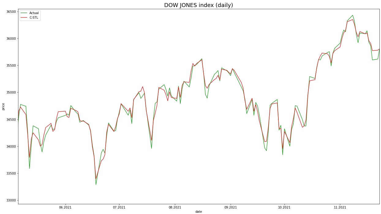
For a clearer visualization of the predictive accuracy, we present a chart contrasting the real versus predicted values of the DOW index. We've sampled a segment from mid-May 2021 to mid-November 2021 for a concise and clearer illustration. This portion encapsulates the performance of our top-performing C-STL model, providing insights into its effectiveness over the illustrated timeframe, particularly in its ability to closely track the actual stock values, thereby reinforcing the quantitative findings presented in Tables 2 and 3. The related chart can be found in Figure 1.

7. Conclusion

7. 1. Summary and Key Findings

In our study on stock index forecasting, we explored the effectiveness of various predictive models. Our analysis revealed that recursive models generally outperformed non-recursive models in terms of predictive accuracy. This trend was particularly notable in the performance of the C-STL model, which demonstrated superior forecasting capability across the Nasdaq 100, Dow, and Dax indices. The C-STL model, utilizing a hybrid approach of CEEMDAN and STL decomposition, consistently showed lower MAPE scores, indicating its higher accuracy. This finding underscores the value of recursive models, especially those involving sub-component analysis, in stock market forecasting. The results highlight the potential of these models in capturing complex market dynamics more effectively than traditional non-recursive approaches.

7. 2. Future Directions

Future research directions should focus on expanding the application of the C-STL model to a wider range of stock indices and market conditions. Investigating ways to enhance the computational efficiency of the C-STL model would also be beneficial, allowing for more extensive testing and refinement. Further exploration into the model's adaptability and robustness in different economic scenarios would contribute significantly to the field of stock market forecasting, balancing theoretical insights with practical utility.

ACKNOWLEDGEMENTS

This research was undertaken as part of my Ph.D. studies under the guidance of Prof. Dr. Bazil Pârv at the Faculty of Mathematics and Computer Science, Babeș-Bolyai University. My sincere thanks to Prof. Pârv for his invaluable support and mentorship.

References

[1] E. F. Fama, "Efficient capital markets: A review of theory and empirical work," The Journal of Finance, vol. 25, no. 2, pp. 383-417, 1970. View Article
[2] B. G. Malkiel, "A Random Walk Down Wall Street: The Time-Tested Strategy for Successful Investing," W.W. Norton & Company Ltd., 2021.
[3] A. Timmermann and C.W.J. Granger, "Efficient market hypothesis and forecasting," International Journal of Forecasting, vol. 20, no. 1, pp. 15-27, 2004. ISSN 01692070. doi: 10.1016/S0169- 2070(03)00012-8. View Article
[4] S. Mokhtari, K. K. Yen and J. Liu, "Effectiveness of Artificial Intelligence in Stock Market Prediction based on Machine Learning," International Journal of Computer Applications, vol. 183, no. 7, pp. 1-8, 2021. View Article
[5] E. F. Fama, "Random walks in stock market prices," Financial Analysts Journal, vol. 51, no. 1, pp. 75-80, 1995. View Article
[6] D. Durusu-Ciftci, M. S. Ispir, and D. Kok, "Do stock markets follow a random walk? New evidence for an old question," International Review of Economics and Finance, vol. 64, pp. 165-175, Nov. 2019. ISSN 1059-0560. doi: 10.1016/j.iref.2019.06.002. View Article
[7] A. M. Rather, A. Agarwal, and V. N. Sastry, "Recurrent neural network and a hybrid model for prediction of stock returns," Expert Systems with Applications, vol. 42, no. 6, pp. 3234-3241, Apr. 2015. ISSN 0957-4174. doi: 10.1016/j.eswa.2014.12.003. View Article
[8] Y. Chen and Y. Hao, "A feature weighted support vector machine and K-nearest neighbor algorithm for stock market indices prediction," Expert Systems with Applications, vol. 80, pp. 340-355, Sep. 2017. ISSN 0957-4174. doi: 10.1016/j.eswa.2017.02.044. View Article
[9] W. Bao, J. Yue, and Y. Rao, "A deep learning framework for financial time series using stacked autoencoders and long-short term memory," PLoS ONE, vol. 12, no. 7, Jul. 2017. ISSN 1932-6203. doi: 10.1371/journal.pone.0180944. View Article
[10] C. H. Su and C. H. Cheng, "A hybrid fuzzy time series model based on ANFIS and integrated nonlinear feature selection method for forecasting stock," Neurocomputing, vol. 205, pp. 264-273, Sep. 2016. ISSN 1872-8286. doi: 10.1016/j.neucom.2016.03.068. View Article
[11] J. L. Ticknor, "A Bayesian regularized artificial neural network for stock market forecasting," Expert Systems with Applications, vol. 40, no. 14, pp. 5501-5506, 2013. ISSN 0957-4174. doi: 10.1016/j.eswa.2013.04.013. View Article
[12] N. E. Huang, Z. Shen, S. R. Long, M. C. Wu, H. H. Shih, Q. Zheng, N.-C. Yen, C. C. Tung, and H. H. Liu, "The empirical mode decomposition and the Hilbert spectrum for nonlinear and non-stationary time series analysis," Proceedings of the Royal Society of London. Series A: Mathematical, Physical and Engineering Sciences, vol. 454, pp. 903-995, 1998. View Article
[13] M. E. Torres, M. A. Colominas, G. Schlotthauer, and P. Flandrin, "A complete ensemble empirical mode decomposition with adaptive noise," in Proceedings of the 2011 IEEE International Conference on Acoustics, Speech and Signal Processing (ICASSP), pp. 4144-4147, 2011. View Article
[14] Z. Jin, Y. Yang, and Y. Liu, "Stock closing price prediction based on sentiment analysis and LSTM," Neural Computing and Applications, vol. 32, no. 13, pp. 9713-9729, Jul. 2020. ISSN 1433-3058. doi: 10.1007/s00521-019-04504-2. View Article
[15] H. Rezaei, H. Faaljou, and G. Mansourfar, "Stock price prediction using deep learning and frequency decomposition," Expert Systems with Applications, vol. 169, May 2021. ISSN 0957-4174. doi: 10.1016/j.eswa.2020.114332. View Article
[16] P. Lv, Q. Wu, J. Xu, and Y. Shu, "Stock Index Prediction Based on Time Series Decomposition and Hybrid Model," Entropy, vol. 24, no. 2, Feb. 2022. ISSN 1099-4300. doi: 10.3390/e24020146. View Article
[17] R. B. Cleveland, W. S. Cleveland, J. E. McRae, and I. Terpenning, "STL: A seasonal-trend decomposition," J. Off. Stat., pp. 3-73, 1990.
[18] J. Senoguchi, "Stock Price Prediction through STL Decomposition using Multivariate Two-way Long Short-term Memory," 2022. doi: 10.32996/jcsts [Online]. Available: https://creativecommons.org/licenses/by/4.0/. View Article
[19] H. He, S. Gao, T. Jin, S. Sato, and X. Zhang, "A seasonal-trend decomposition-based dendritic neuron model for financial time series prediction," Applied Soft Computing, vol. 108, Sept. 2021. ISSN 1568-4946. doi: 10.1016/j.asoc.2021.107488. View Article
[20] R. H. Shumway and D. S. Stoffer, Time Series Analysis and Its Applications. Springer, 2017. View Article
[21] T. Shiba and Y. Takeji, "Asset Price Prediction Using Seasonal Decomposition," Financial Engineering and the Japanese Markets, vol. 1, pp. 37-53, 1994. View Article
[22] Scikit-learn: Machine Learning in Python [Online]. Available: View Article
[23] Yahoo Finance [Online]. Available: View Article
[24] yfinance Python package [Online]. Available: View Article
[25] sklearn.metrics: Metrics and scoring: quantifying the quality of predictions [Online]. Available: View Article
[26] sklearn.svm.SVR: Epsilon-Support Vector Regression [Online]. Available: View Article