Journal of Machine Intelligence and Data Science (JMIDS)

1. Introduction

Copulas are principally utilized for modelling dependencies in multivariate distributions. Their properties have been increasingly exploited in numerous types of scientific investigations; for instance, the reader may refer to Chao et al. [1], Carrera et al. [2] and Chen et al. [3] for recent advances in the area of artificial intelligence. The key idea behind copulas is that the joint distribution of two or more variables can be represented in terms of their marginal distributions and a specific correlation structure. As a measure of dependence, they have for instance found applications in reliability theory, signal processing, geodesy, hydrology and medicine. Results involving empirical bivariate copula densities are discussed in this paper.

Let F(x₁,x₂ ) be the joint cumulative distribution function of random variables X₁ and X₂ having continuous marginal distribution functions F₁ (x₁) and F₂ (x₂ ). According to Sklar [4], there exists a unique bivariate copula C:I₂↦I (the unit interval) such that

(1)

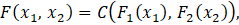
where C(⋅,⋅) is a joint cumulative distribution function having uniform marginals. Conversely, for any continuous cumulative distribution function F¹ (x¹ ) and F² (x² ) and any copula C, the function F defined in Equation (1) is a joint distribution function with marginal distributions F¹ and F².

Sklar's theorem provides a technique for constructing copulas. Indeed, the function

(2)

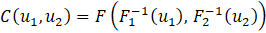
is a bivariate copula, where the quasi-inverse F_i^(-1) for i=1,2 is defined by

(3)

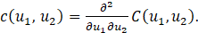
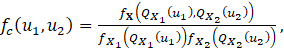
We shall denote the probability density function corresponding to the copula C(u₁,u₂ ) by

(4)

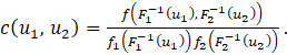
The following relationship between the joint density function f(⋅,⋅) and the copula density function c(⋅,⋅) can readily be obtained from Equation (1):

(5)

where f₁ (x₁ ) and f₂ (x₂ ) respectively denote the marginal density functions of X₁ and X₂. Accordingly, the copula density function can be expressed as follows:

(6)

The proposed approaches to estimating copula density functions are summarized in Sections 2 and 3. The estimation of a joint density function in terms of marginal distributions and a copula density estimate is discussed in Section 4. Three illustrative examples are provided in the last section.

2. Copula Density Based on Kernel Density Estimation

On applying the kernel density estimation (kde) method to a given bivariate dataset, one can obtain an estimate of the bivariate probability density of X. In light of Equation (6), the copula density can be represented as follows:

(7)

where f_X can be estimated by a bivariate kde and Q_Xi (⋅) denotes the quantile function. The marginal density function of each variable can be obtained by determining their respective kernel density estimates. The inverse cdfs Q_X1and Q_X2 can be determined in polynomial form by making use of a moment-based method or the method of least squares.

3. A Moment-based Bivariate Polynomial Approximation of the Copula Density

Once a copula density is determined from Equation (7), it can be approximated by the product of a base density and a bivariate polynomial whose coefficients are obtained from the joint moments associated with the copula density.

The proposed procedure for achieving this is described in the next result.

Result 1 Let f_X (x₁,x₂ ) be the density function of a bivariate continuous random vector X=(X₁,X₂ ) defined in the rectangle (l₁,u₁ )×(l₂,u₂ ), whose joint moments are

(8)

Let ψ(x₁,x₂) be an initial joint density estimate, whose joint moments are

(9)

Assuming that the sequence μ_X (i,j), i=0,1,2,…, j=0,1,2, uniquely defines the distribution of X, the density function of X can be approximated by

(10)

where ξ_i,j can be determined by letting

(11)

h=0,1,…,n;g=0,1,…,n, or equivalently,

(12)

h=0,1,…,n; g=0,1,…,n. Thus, we can obtain the polynomial coefficients ξ_i,jand f_n (x₁,x₂ ) from the moments of f_X (⋅) and ψ(⋅) by solving the linear system specified by Equation (12).

The degree n used in the polynomial adjustment should be selected so that f_n provides an accurate approximation to the estimate of the copula density, which can be determined for instance by evaluating their integrated squared differences.

4. Estimating a Joint Density from the Marginal Density Estimates and the Copula Density

On applying Equation (5), that is,

(5)

one can determine the joint density where for instance, c(⋅,⋅) could be taken as a Bernstein copula density which is described in Sancetta and Satchell [5].

Suppose that observations are available on the random variables X₁ and X₂. The marginal densities f₁ (x₁ ) and f₂ (x₂) are estimated and a Bernstein's copula density of high order is determined. A joint density estimate of (X₁,X₂) can then be obtained via Equation (5).

5. Applications

The results are applied to two stocks’ closing prices as well as a stock’s price and its running maximum.

5.1. Copula Density Estimation Methodologies Applied to Two Stocks

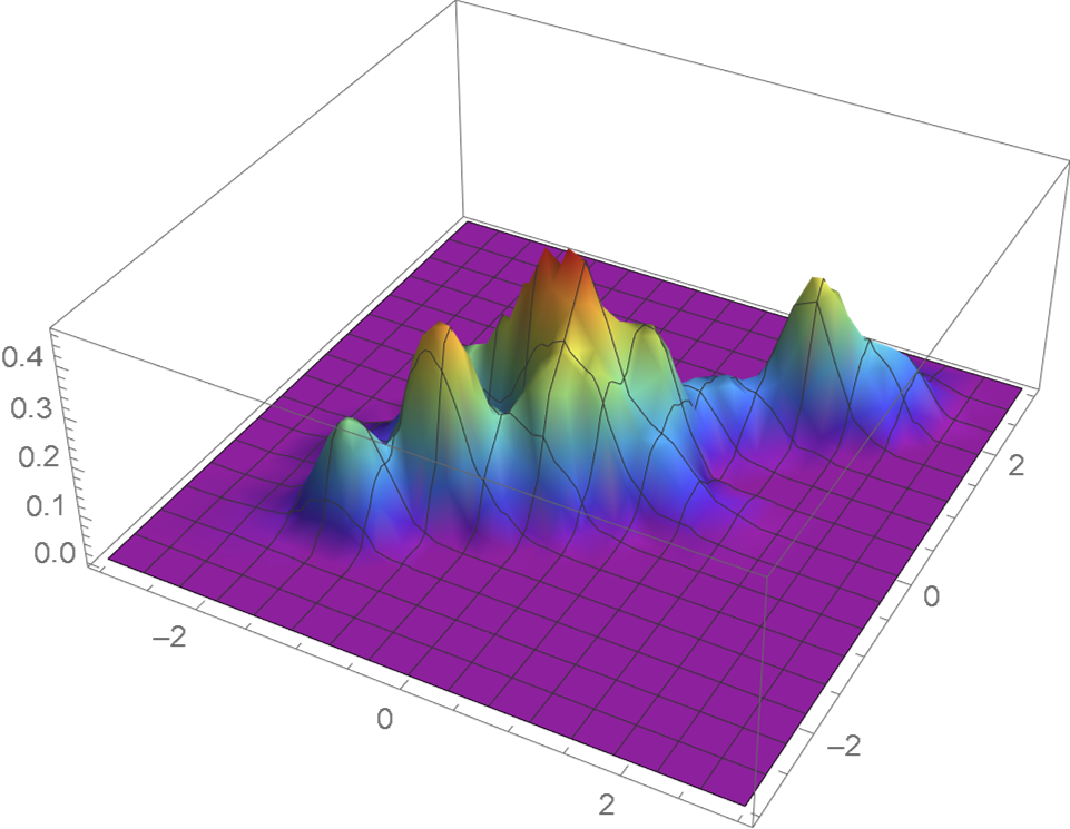
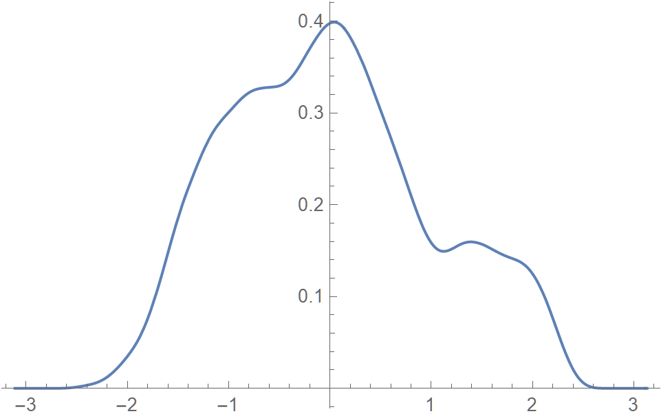
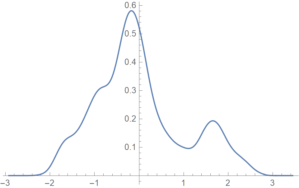
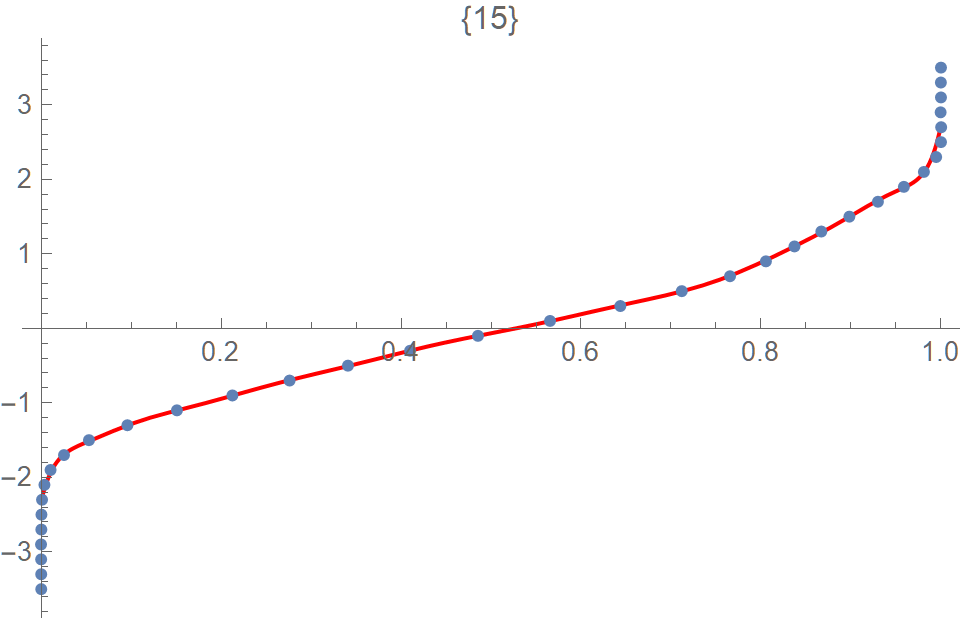
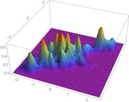
The two stocks selected are GOOG (Alphabet Inc.) and AAPL (Apple Inc.). The bivariate data are the daily closing prices of (GOOG, AAPL) in 2019. Each component of the data has been standardized. The joint KDE of X, the marginal densities of X₁ and X₂ and the corresponding cdf inverses are displayed in Figures 1-5.

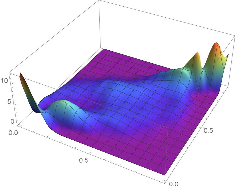
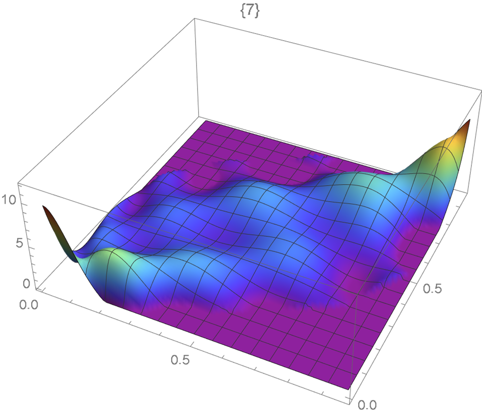
The resulting KDE based (Section 2) and moment-based (Section 3) copula densities plotted in Figures 6 and 7 are seen to be similar.

5.2. Determination of a Joint Density Estimate from the Marginal Density Estimates and the Copula Density

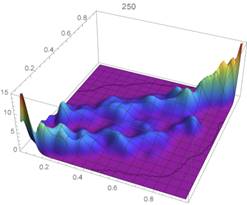
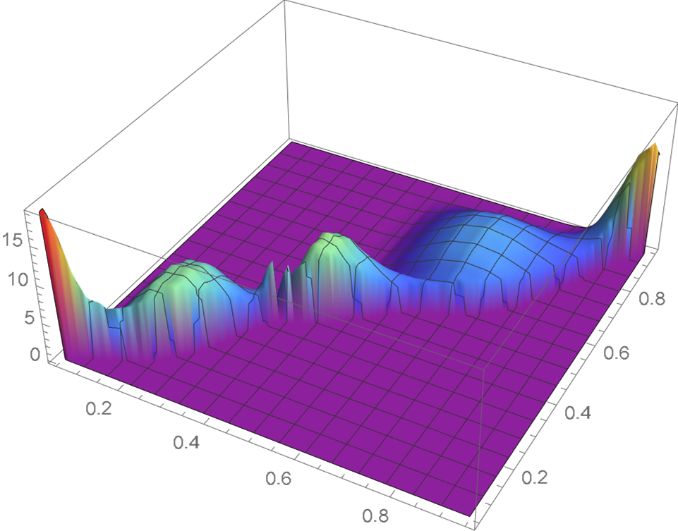
Using the two stocks’ standardized data, a Bernstein’s copula density of degree 250, which is shown in Figure 8, is utilized as an estimate of the underlying copula density. The density estimate (Figure 9) resulting from the application of the methodology described in Section 4 and a KDE (Figure 10) exhibit very similar features.

5.3. Copula Associated with a Brownian Motion Process and Its Running Maximum

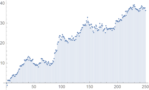
The data consists of the daily closing prices of AC.TO (Air Canada) during 2019. To relate the data to a standard Wiener process, the first data point should be zero, the differences between successive observations should ideally often change signs and have a variance of one, and there should be one unit of time between successive observations. Hence the following transformation is used.

Let U₁,U₂,…,U_n denote the closing prices and V₁,V₂,…,V_n-1 be the differences between successive closing prices, that is, V_i=U_i+1-U_i; denoting by σ_D the standard deviation of the differences V₁,V₂,…,V_n-1, the following transformation is applied W_i=(U_i-U₁)/σ_D and the resulting data is denoted by W₁,W₂,…,W_n.

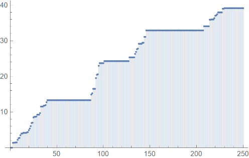
Let Z_i be the i^th running maximum, that is, Z_i="Max"\{W₁,W₂,…,W_i \}, i=1,2,…,n. Then, the resulting bivariate data, (W_i,Z_i ), i=1,2,…,n, has the features of a Brownian motion process and its running maximum.

The W_i’s and Z_i’s are plotted in Figures 11 and 12. The resulting copula density as obtained by applying the methodology described in Section 2, is shown in Figure 13.

6. Conclusion

As copula density estimates are usually expressed in complicated forms, the bivariate polynomial approximation that is proposed in this paper ought to prove more suitable for reporting purposes. Approximations by means of Bernstein polynomials and the kernel density estimation approach are discussed as well. Additionally, a flexible technique for estimating joint density functions is introduced. The proposed methodologies were successfully applied to two stocks' closing prices as well as a set of observations and its running maximum.

References

[1] M. Chao, S. Z. Xin, and L. S. Min, "Neural network ensembles based on copula methods and distributed multiobjective central force optimization algorithm," Engineering Applications of Artificial Intelligence, vol. 32, pp. 203-212, 2014. View Article
[2] D. Carrera, R. Santana, and J. A. Lozano, "Vine copula classifiers for the mind reading problem," Progress in Artificial Intelligence, vol. 5(4), pp. 289-305, 2016. View Article
[3] T. Chen, S.-S. He, J.-Q. Wang, L. Li, and H. Luo, "Novel operations for linguistic neutrosophic sets on the basis of Archimedean copulas and co-copulas and their application in multi-criteria decision-making problems," Journal of Intelligent & Fuzzy Systems, vol. 37(2), pp. 2887-2912, 2019. View Article
[4] M. Sklar, "Fonctions de répartition à n dimensions et leurs marges," Publications de I'Institut de statistique de I'Université de Paris, vol. 8, pp. 229-231, 1959.
[5] A. Sancetta and S. Satchell, "The Bernstein copula and its applications to modelling and approximations of multivariate distributions," Econometric Theory, vol. 20, pp. 535-562, 2004. View Article