Journal of Machine Intelligence and Data Science (JMIDS)

1. Introduction

Environmental monitoring is very important to help determine the ecological health of an area. For example, animal population, foliage health, local weather information, air pollution, and water quality are all important factors that can be monitored using unmanned ground vehicles (UGV) [1-4]. These missions require a long-term process and are best done remotely, as a result, any UGVs sent into the field to study the environment need to survive for long periods of time and travel far distances [5]. With Ray [6], solar harvesting was used in order to have the “cool robot” SPUGV travel 500 km across Antarctica to conduct and run scientific experiments. Areas such as Antarctica have consistently high sources of solar irradiance (SI) so path planning towards a goal was focused on rough terrain and obstacle avoidance. Others such as Plonski [7,8] developed an algorithm to construct a solar map for a defined area using an SPUGV for future path planning in the constructed solar map. Kaplan [9,10] developed a time-optimized path planning algorithm for a SPUGV in a known solar environment so that the robot minimized travel time while also moving through high SI points on its way to the goal in order to increase the battery life of the SPUGV. All of the approaches require significant planning and mapping of an area in order for the SPUGV to navigate through it. Also, as Plonski [7] discussed, the solar environment in an area is constantly changing as the sun moves, so any solar mapping data may be inaccurate by the time the robot begins path planning.

Despite the research for path planning in known solar environments, little has been done for path planning in unknown solar environments. Current path planning techniques need detailed solar environment information for the SPUGV to traverse an environment which is not always feasible or reasonable. Solar environments are constantly changing each day and throughout the year, therefore, path planning in an unknown solar environment would make environmental monitoring missions using UGV’s a more viable option. To this end, we propose a cost function switching (CFS) algorithm developed to maximize the battery life of a SPUGV as it travels to points of interest in an unknown solar environment. The major contribution of this work is that the CFS algorithm eliminates the need for prior solar information of an area for SPUGV path planning in environmental monitoring missions.

2. Problem Definition

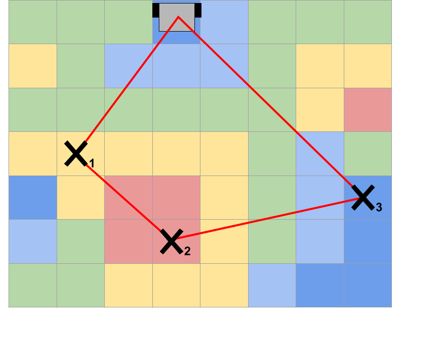
Suppose a SPUGV is placed into an environment with a variety of SI intensities with the task to reach multiple points of interest and then to return to the starting position with the maximum battery life achievable. Figure 1 demonstrates a discretized global solar map with the SI values ranging from high in red, to low in dark blue where X₁, X₂, and X₃ are points of interest in sequential order.

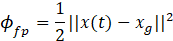
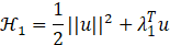
The problem can be defined as two path cost functions that seek to minimize the amount of energy expended when either moving towards a point of interest or a SI peak to charge. The first cost function J₁ seeks to minimize the control input cost with the goal position being the terminal cost. The J₂ cost function also minimizes the path cost of the input velocity, however, the terminal cost is a sampled local SI peak instead of a point of interest or goal position. With the SPUGV’s current position , the goal position , the local energy peak position , and the control input , we use a first-order robot dynamics and the control input is saturated by u_max as constraints. Then the optimization problem is formulated by

(1)

(2)

where the symbol ϕ_fp is the terminal cost of the goal and ϕ_fp is the terminal cost of the local SI peak as follows:

(3)

(4)

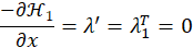
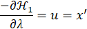
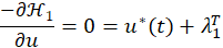
With the cost functions defined, the optimal solution u^* can be obtained by two Hamiltonian equations. The Hamiltonian for J₁ is shown in equation (5), which looks similar to the Hamiltonian for J₂.

(5)

(6)

(7)

(8)

Equations (6) and (7) can be discretized and combined with equation (9) to find the optimal control input u^* in discrete time intervals. Equations (6) and (7) can be discretized and combined with equation (9) to find the optimal control input u^* in discrete time intervals.

(9)

(10)

(11)

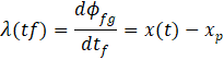
Likewise, for equation (11), equation (7) can be rewritten into equation (12).

(12)

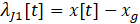
Because the costate variable λ(t) is unchanging for both J1 and J2, the problem is defined by four equations that provide the optimal path for J₁ and J₂ which are shown in equations (13) through (16). Note that equation (13) is the costate variable definition for J1 and equation (14) for J₂.

(13)

(14)

(15)

(16)

At each time step, the optimization problems in (1) and (2) can be solved based on the Hamiltonian approach (5) - (16) in a receding-horizon manner [11 - 17]. This implies that after the local SI measurement is taken using the onboard sensor, the SPUGV can determine where to go with a horizon length T, which is repeated at each time. This receding-horizon technique will enable the SPUGV to cope with a realistic scenario where a global SI map is not available and hence, the SPUGV needs to make a decision only with local information.

In this case, the challenging part is how to determine the appropriate control input between the two optimal solutions. The performance will vary depending on the switching logic for the control input. In what follows, we thus investigate the switching algorithm between the two different control inputs.

3. Main Result

3. 1. CFS Algorithm for Path Planning

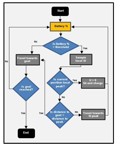
In order to maximize the battery, the robot needs to prioritize either charging the battery or reaching the goal at any given time. This is our scenario and the proposed CFS algorithm will determine the instance of switching between the two optimal control inputs obtainable by solving for J₁ or J₂. We utilize a battery threshold as a switching criteria between the two functions. For instance, if the battery threshold is set to 60% of the max battery and the battery reaches 60%, then the robot begins searching for nearby solar irradiance peaks. This is done with a sensing algorithm to determine the highest irradiance value with the closest distance to the goal. When a peak SI value is found, the robot will go towards the peak to charge the battery. The process of finding a SI peak is done continuously until the SPUGV reaches the local peak. The decision is made by observing four different variables, the SI at the current location, the SI at the measured peak, the distance from the current location to the peak, and the distance between the current location and the goal. If the robot has a lower measured SI than the peak and the distance to the peak is smaller than the distance to the goal, then the robot will move to the peak value as depicted in the flow chart shown in Figure 2. If the robot has a SI larger than the measured peak, the robot is at a local maximum and will stay there until charged to a set upper charging threshold. If the goal distance is less than the distance to the peak, the robot will just go towards the goal. If none of these conditions are met, the robot will continue towards the goal to avoid getting stuck along the path.

3. 2. Sensing Algorithm

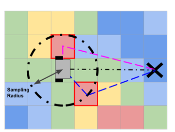
Choosing a single local SI peak among multiple of them requires another algorithm to detect and evaluate the SI around it. The sensing algorithm takes samples of a set sampling radius and step size and creates a sampling matrix of local SI values. An example sampling matrix is shown in Figure 3, where the local sampled SI values also include the SI of the robot’s current position. Efficient evaluation of the samples was done by incorporating a statistical threshold so that only the highest SI values are observed. The threshold for peaks was set at 2 standard deviations from the mean of SI samples so that only the top 5% of SI in the local region are considered. The results from the thresholded sampling algorithm are multiple high SI peaks and their locations. Because the robot can only go towards one of the points, the sampling algorithm evaluates the SI at each local peak, the distance between the robot's current positions, and the distance between the peak and the goal position. By having distance as a method for determining the local max SI peak, the algorithm prioritizes energy peaks that are closer to the goal which prevents the robot from diverging away from the goal while searching for energy.

Figure 3 visualizes what the local sample from the robot looks like. The red squares indicate highest SI peaks while blue squares indicate lowest SI peaks. As shown in Figure 3, the SPUGV does not see the global solar information and can only see within the sample radius. With the thresholding, only two peaks would be considered for the local peak and therefore can be compared along with the distance directly to the goal from the robot to determine which path to be taken.

4. Simulations

4. 1. CFS Algorithm for Path Planning

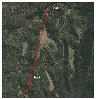
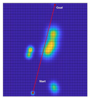
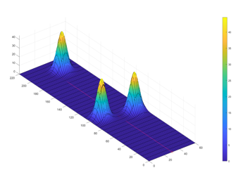
In order to test the application of using the CFS algorithm, two different simulation environments were created. The first environment was mapped in reference to a section of the Santa Fe National Forest in New Mexico, USA. The simulation uses multiple Gaussian distributions of SI that the robot can measure. New Mexico receives an average of 41.6 W/m2 of SI which is reflected in the solar map [18]. The high-intensity regions of the map indicate open areas such as a meadow in the forest with the assumption that the simulation is occurring when the sun is perpendicular to the ground and unchanging throughout the simulation. For simplicity, the simulation assumes that there are no inclination changes or obstacle obstructions that would be seen in the real environment. Researchers such as Engine, Wang and Mei have implemented more realistic vehicle dynamics however this is beyond the scope of this paper [19-21]. The robot chassis chosen for the simulation is the MLT-JR with two IG32 motors, two 2200maH batteries. The solar panel being simulated on the robot is an Eco-Worthy 10 W panel as shown in Figure 4.

In the Santa Fe simulation, the SPUGV traveled from an initial position to a single point of interest. The SPUGV would start and end in a meadow where SI should be found. The distance between the two points was 2.5 km which is within the max distance the SPUGV can travel on one full charge of battery. The simulation was run using both the CFS algorithm and a direct route approach to determine if the battery at the goal position could be improved. The second Santa Fe simulation involved four points of interest on the same solar map as simulation 2. For simulation 2, the SPUGV starts at an initial point and then travels to each point directly, only moving onto goal 3 after arriving at goal 2 and so on. The total distance to travel to all the points sequentially was 2.5 km. The CFS algorithm was also compared to a direct route approach with multiple points of interest. Both simulations use a 5 m sensing radius for the SPUGV.

In order to understand the more detailed path behavior of the SPUGV, small scale lab simulations were created. The lab simulation involves the SPUGV traveling through a flat environment with set SI peaks along its path as shown in Figure 7. Two types of lab simulations were created, 100 meter and 200 meter distance. The same robot and SI max used for the Santa Fe simulations are applied to the lab simulations. Because of the shorter distance, the robot’s battery lasts longer than what is expected in real life so for the lab simulations the battery threshold was increased to 96% compared to 60% in the Santa Fe simulations.

4. 2. Simulation Results

The simulation shown in below demonstrates that the SPUGV using the CFS algorithm will reach the goal position with a significantly higher battery percentage than a direct route to the goal. For simulation 1, the trajectory of the SPUGV heads directly towards the goal until the battery threshold of 60% is met where it begins searching for SI peaks. Figure 8 shows the local peak SI values as bright green triangles. The path clearly shows the robot traveling towards the peak that is closest to the final goal. In the simulation, the CFS algorithm took 166 minutes longer to reach the goal than the direct route, however, the CFS resulted in a 40.7% higher battery percentage at the goal. This shouldn’t be a problem for applications like environmental monitoring, where a sustainable operation of UGVs is much more important than the time taken. Likewise, for the second simulation, the SPUGV took 333 minutes longer to complete the loop but with 70% more battery.

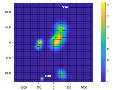
Table 1. Simulation 1 battery and time results.

Algorithm	Time (minutes)	Battery % at tf
None	49	24.2
CFS	215	64.9

Table 2: Simulation 2 battery and time results.

Algorithm	Time (minutes)	Battery % at tf
None	69	0.7
CFS	402	71.0

For the lab simulations, the local trajectory of the SPUGV can be observed, the locally detected SI peaks are red triangles. In simulation 3, the SPUGV can choose between two different equidistant SI peaks of different intensities along its path. The sampling algorithm chooses the highest peak in the SPUGV’s range that is closest to the goal. The resulting trajectory wraps around the peak towards the goal until it reaches a high enough SI peak to charge. In simulation 4, the SPUGV’s ability to travel towards a goal position if it gets close enough to it was tested. As shown in Figure 13, even if a peak position is very close to a goal position, the SPUGV will go towards a goal position. This will prevent the SPUGV from diverging from a goal position to charge if it is close to the goal. In simulation 5, the goal position was moved an additional 100 meters so the SPUGV would need to recharge more than once. At longer distances, the battery difference between a direct and CFS trajectory is much more noticeable as the SPUGV had almost 8% higher battery life with the CFS algorithm.

For the multi-goal simulations in simulation 6 and 7 (Figures 15 and 16, respectively), the SPUGV’s trajectory is not as predictable as a single goal. In this case, the SPUGV was given two goal positions to reach before returning to the start location forming a triangular trajectory when using a direct path. With the CFS the algorithm favored the side of the simulation with more solar irradiance despite it only being able to see SI in a 5 meter radius. One thing to note with the CFS algorithm is that it not only takes longer because the SPUGV needs to charge, but it also limits the mobility of the SPUGV to the local SI peak so it doesn’t overshoot the peak. Throughout the simulations, there can be seen some peaks that the SPUGV doesn’t follow, these peaks are detected but have a small SI value less than 1W/m.

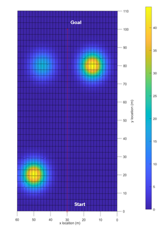
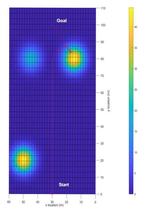
Table 3: Simulation 3 battery and time results.

Algorithm	Time (minutes)	Battery % at tf
None	5	95.1
CFS	25	99.1

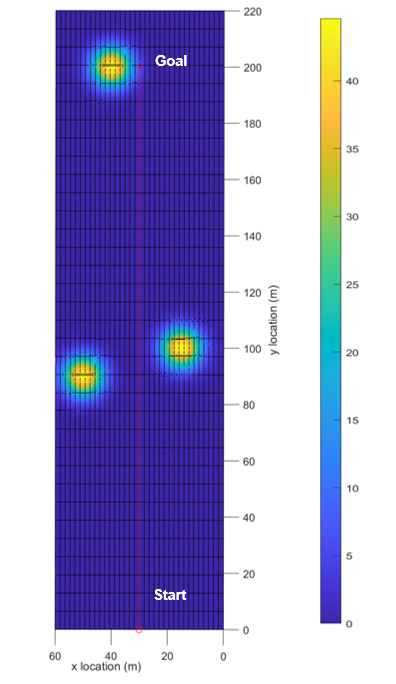
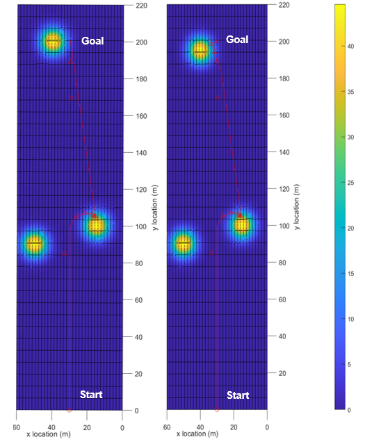
Table 4: Simulation 4 battery and time results.

Algorithm	Final SI Peak distance from goal x location (m)	Time (minutes)	Battery % at tf
None	15	10	89.0
CFS	15	36	94.5
CFS	10	39	93.7

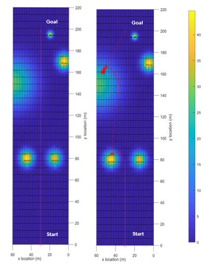
Table 5: Simulation 5 battery and time results.

Algorithm	Time (minutes)	Battery % at tf
None	5	95.1
CFS	25	99.1

Table 6: Simulation 6 battery and time results.

Algorithm	Time (minutes)	Battery % at tf
None	5	95.1
CFS	25	99.1

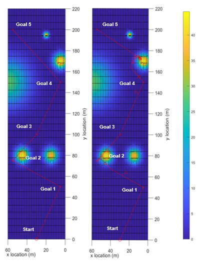
Table 7: Simulation 7 battery and time results.

Algorithm	Time (minutes)	Battery % at tf
None	20	83.5
CFS	71	96.3

5. Conclusion

In this paper, maximizing battery life during the mission such as environmental monitoring in an unknown environment is shown to be effectively done with the proposed CFS algorithm. The proposed method, which prioritizes either the goal point or a local peak of SI depending on the remaining battery, guarantees that it will reach a point of interest with a higher battery life than going directly to a goal and therefore, extend the mission life. The simulations shown demonstrate the versatility of the CFS algorithm in a variety of possible scenarios. As long as a SI peak is detectable along the path of the SPUGV, the battery life will be significantly higher than just reaching a goal.

References

[1] M. Dunbabin, and L. Marques, "Robotics for Environmental Monitoring," IEEE Robotics & Automation Magazine Volume 19(1), pp. 24-39, 2012 View Article
[2] N. Olmado, B. Fisseha, W. Wilson, M. Barczyk, H. Zhang, M. Lipsett, "An automated vane shear test tool for environmental monitoring with unmanned ground vehicles," Journal of Terramechanics 91, pp. 53-63, 2020 View Article
[3] S. Bonadies, A. Lefcourt, and S. Gadsden, "A survey of unmanned ground vehicles with applications to agricultural and environmental sensing," SPIE Commerical + Scientific Sensing and Imaging, 2016 View Article
[4] Committee on Army Unmanned Ground Vehicle Technology, et al. "Technology Development for Army Unmanned Ground Vehicles," National Academies Press, pp. 17-19, 2002
[5] Jones, Julia PG, G. Asner, S. Butchart, K. Karanth, "The 'why','what'and 'how'of monitoring for conservation," Key topics in conservation biology 2, pp. 327-343, 2013 View Article
[6] L. Ray, J. Lever, A. Streeter, A. Price, "Design and power management of a solar‐powered "cool robot" for polar instrument networks," Journal of Field Robotics 24.7, pp. 581-599, 2007 View Article
[7] Plonski, Patrick A., Joshua Vander Hook, and Volkan Isler. "Environment and solar map construction for solar-powered mobile systems," in IEEE Transactions on Robotics 32.1, pp. 70-82, 2016 View Article
[8] P. Plonski, T. Pratap, and I. Volkan. "Energy‐efficient path planning for solar‐powered mobile robots," Journal of Field Robotics 30.4, pp. 583-601, 2013 View Article
[9] A. Kaplan, N. Kingry, P. Uhing, R. Dai, "Time-optimal path planning with power schedules for a solar-powered ground robot," IEEE Transactions on Automation Science and Engineering 14.2, pp. 1235-1244, 2016 View Article
[10] A. Kaplan, P. Uhing, N. Kingry, R. Dai, "Integrated path planning and power management for solar-powered unmanned ground vehicles," IEEE International Conference on Robotics and Automation, 2015 View Article
[11] K. Lee, S. Martínez, J. Cortés, R. H. Chen, and M. B. Milam, "Receding-horizon multi-objective optimization for disaster response," In 2018 Annual American Control Conference (ACC), pp. 5304-5309. IEEE, 2018. View Article
[12] R. H. Kabir, and K. Lee, "On the ergodicity of an autonomous robot for efficient environment explorations," In Dynamic Systems and Control Conference, vol. 84287, p. V002T31A003. American Society of Mechanical Engineers, 2020.
[13] R. H. Kabir, and K. Lee, "Receding-horizon ergodic exploration planning using optimal transport theory," In 2020 American Control Conference (ACC), pp. 1447-1452. IEEE, 2020. View Article
[14] R. H. Kabir, and K. Lee, "Wildlife monitoring using a multi-uav system with optimal transport theory," Applied Sciences, vol. 11, no. 9, p. 4070, 2021. View Article
[15] R. H. Kabir, and K. Lee, "Efficient, decentralized, and collaborative multi-robot exploration using optimal transport theory," In 2021 American Control Conference (ACC), pp. 4203-4208. IEEE, 2021. View Article
[16] K. Lee, and R. H. Kabir, "Density-aware decentralised multi-agent exploration with energy constraint based on optimal transport theory," International Journal of Systems Science, pp. 1-19, 2021. View Article
[17] W, Kyon, S, Han, S. H. Han, "Receding Horizon Control Model Predictive Control for State Models," Springer London, 2005
[18] Direct Solar Irradiation (2020) [Online]. Available: View Article
[19] M. Engin, and D. Engin, "Optimization Controller for Mechatronic Sun Tracking System to Improve Performance," Sage Jounrals: Advances in Mechancial Engineering, vol. 5, 2013 View Article
[20] G. Wang, M.J. Irwin, P. Berman, H. Fu, T. Porta, "Optimizing sensor movement planning for energy efficiency," ISLPED '05, 2005 View Article
[21] Y. Mei, Y. Lu, C.S.G. Lee, Y.C. Hu, "Energy-Efficient Mobile Robot Exploration," IEEE International Conference on Robotics and Automation, 2006
[22] L. Strebe, K. Lee, "Battery Energy Maximization for Solar Powered Unmanned Ground Vehicle," International Conference on Control, Dynamic Systems, and Robotics, 2022 View Article