Journal of Machine Intelligence and Data Science (JMIDS)

1. Introduction and Previous Work

Autonomous driving has been on the receiving end of a lot of attention and interest with the resurgence of artificial intelligence (AI) techniques due to more potent computing hardware. Although many of the artificial intelligence techniques today root in research conducted decades ago, they have only become viable and practical options in the past few years with modern computers orders of magnitude faster than those of the era where these techniques were conceptualized. The reason autonomous driving is so intertwined with AI, owes to the complexity of the problem. It would be near impossible to create a definitive set of rules that would undertake all the navigating and manoeuvring tasks for a vehicle. To put that into perspective, recent publications in vehicle systems using classical controllers can be examined. These studies [1, 2, 3, 4] are perfect examples of the limits of what even modern analytical controllers can achieve. While being robust and even useful in many driving scenarios, they do not provide any versatility and fail in case of any deviation from the situations they are designed for. These deviation scenarios are plentiful in normal day-to-day driving. Adding fuel to the fire, is the fact that automated vehicles are expected to be deployed alongside human drivers as they will not replace their human driven counterparts overnight, in which case erratic behaviour of human drivers and the inappropriate infrastructure are two major impediments.

Having realized the challenges, one might ask considering all the encumbrance, is autonomous driving research even worth it? According to statistics released by U.S. National Highway Traffic Safety Administration (NHTSA) [5, 6] in 2015, the surveys indicate that out of the 2,189,000 reported traffic accidents, 94% ± 2.2% were due to human error, and grievously 35,092 were fatal. The same document points out that 41% ± 2.2% were due to human recognition error which has statistical significance. The promise of automated driving can be enumerated as:

1. Affordable long-range transportation for the public.
2. Personal transportation for individuals with disabilities.
3. Diminishing of traffic casualties associated with human error.
4. Minimization of harmful exhaust emissions. [7]

Having established the challenges of automated driving, one solution is tackling the problem with empirical methods such as machine-learning/AI techniques. The question then becomes what techniques work best, as there are a variety of techniques available. Studies such as one by Zhang et al. [8] uses chaining neural networks to predict longitudinal motion of vehicles using drive-cycles but does not consider context or lateral motion which are two integral parts of driving. Similarly, in the study conducted by Sun et al. [9] while multiple CVPMs are compared, the approach does not consider multiple variables and extension of the same approach for multiple variables will not encompass the dependencies between those variables. Likewise, Thorsell’s [10] approach can make single drive cycle predictions without considering spatial information. There are many other studies following the same principles, and that is what makes this study unique. This approach considers context, can adapt to the situation, and the predictions can be done on any variable while their dependencies are conserved. However, for the sake of ease of comparison, this study also focuses on velocity predictions. This study builds on a suite of studies that focus on different driving scenarios, adapting a new solution for every situation. Roundabouts are subject to a new emergence in developing urban landscape as they provide a passive, smarter way to control the traffic as opposed to traffic light-controlled intersections. Roundabouts are adaptive to the flow and temporal changes in traffic, but in turn poses a threat to inexperienced drivers who are not acquainted with roundabout driving, often causing a chain reaction in traffic accidents. The following sections will go over the basics and the background of the approach, then the strategy is discussed, and finally results are declared and discussed, followed by conclusions and future work.

2. Background

This study builds on dynamic Bayesian network as a core of its hybrid approach. DBN is a powerful probabilistic inference tool that can incorporate traffic rules directly from expert knowledge, however, to compensate for its lack of ability to make accurate predictions on continuous variables, a contractor data-driven sequence prediction method, dubbed CVPM was used. Figure 1illustrates an overview.

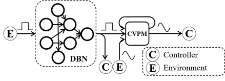
In Figure 1, the case of controller is a hypothetical one and as it will be discussed in the conclusion, this prediction strategy is a prime target to be used with model predictive controllers (MPCs) to provide them with accurate state predictions. The other main components are the DBN, and the CVPM.

2. 1. Dynamic Bayesian Network

A Bayesian network [11] is a graphical representation of probabilistic variables where the connections serve as dependencies between those variables. In a driving context, most of the variables can be categorized as probabilistic and their values can be classified into mixture distributions. As an example, a traffic light signal has 3 states (4 if considering advanced left). Similarly, ‘current lane of driving’ has a limited number of states. Even in some cases, where the actual value of a continuous variable is not critical, continuous variables can be turned into a mixture distribution by introducing semantic rules. For instance, for a variable such as distance, anything past a threshold can be dubbed “far” and below that threshold “near”. As far as mixture distributions and discrete variables are concerned, DBN is a powerful tool that can obtain likelihood of each variable taking a specific state given a set of conditions. As mentioned in the introduction, the purpose of the perception middleware is to be able to understand traffic participants behaviour and incorporate expert knowledge into understanding the environment. This approach is replicating the learning process of driving for a human. A human driver is not adequately equipped to be able to measure distances and speeds numerically but will always know, semantically, whether an object is too far or near, or too fast or slow. Also, a human driver by knowledge and experience knows that the lane in which a vehicle enters an intersection in will govern its destination. There is always a degree of uncertainty, but the human driver can adapt their initial assumption if given a set of observations.

Bayesian networks can be classified as expert systems in the sense that the topology can be defined by an expert which will provide the network with an initial understanding of the relationship between variables. They are also a data-driven approach that can learn from large datasets quickly. The dataset will be stored as sets of Gaussian normal distributions of P(A|Pa(A)), where A is a probabilistic variable and Pa(A) is the set of its parents (i.e., set of variables with an edge toward A). Once fully learned, any joint or conditional probability between variables can be computed. The learning process in Bayesian networks is done through EM algorithm, a descendent of the forward-backward algorithm. In this algorithm a set of Gaussian normal distributions are fitted to mixture distributions by generating n random Gaussian distributions, finding the likelihood of each sample belonging to each distribution and then updating the distribution properties based on classed samples. [12] DBNs are Bayesian networks with temporal nodes which are variables with values from the next time-slice in the training. However, not every variable in a driving context can be represented as a mixture distribution. Variables such as speed are continuous, and their value is often desired. DBN is not adequately equipped to make predictions for continuous variables, hence there is the need for a CVPM.

2. 2. Continuous Variable Prediction Module

The continuous variable prediction module can be any data-driven sequence prediction method. In machine learning realm, primitively a feed-forward neural network can be equipped with a feedback loop and unit delays to become a recurrent neural network (RNN). An RNN can then be trained to take a short history of the variable as the input and produce predictions for the next time slice. By repeating the cycle, assuming the predicted value as the true current value and cascading the history one step back, each the prediction can be extended to an arbitrary horizon. Although it is common knowledge that as the horizon becomes larger the accuracy suffers because of the compounding effect of the errors.

RNNs are known to struggle with the vanishing gradient problem. The vanishing gradient problem is, in essence the stoppage of training due to the shrinking error gradient in the back-propagation algorithm. The opposite of gradient explosion problem is where the large gradient will cause the training to diverge from the global optimum. A solution to this problem is using modified recurrent neural networks such as the gated recurrent unit networks (GRU), or long short-term memory networks (LSTM). The main difference between these modified versions versus the vanilla RNN is presence of trainable gates. These gates named forget, input, and output for LSTM, and reset, and update, for GRU, control the flow of data (and cell state for LSTM) to segregate and prioritize important new information. This ability is specifically useful for cases such as natural language processing or visual target tracking where parts of the input are ineffectual. Though, it is important to note, by adding these trainable gates, the training of a network becomes slower, and most likely, if the RNN does not run into the aforementioned problems, epoch-for-epoch yields little accuracy in comparison. In other words, it is expected for RNN to be the most efficient technique of the bunch in absence of vanishing/exploding gradient problem.

3. Implementation Strategy and Results

As mentioned in the previous section, the approach taken in this study is a data-driven one. The first step toward developing a data-driven prediction strategy is to understand the dataset and know what variables are available to work with. As available datasets are often lacking in useful data as data collection is generally time consuming and difficult to the point where it is completely implausible, the refuge is to simulation. In this study, a simulation environment was implemented in SUMO [13]. To clarify, the only difference between using real data and simulation for the case of making predictions is extra pre, and post processing steps which are trivial to the core of the prediction methodology. However, it is important to note, the previous statement only applies to law-abiding norm. If the networks are not trained for car crashes, or aggressive manoeuvres, they are not able to predict such occurrences.

3. 1. Simulation in SUMO

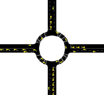
The scope of this study is roundabout driving which is emerging in developing cities. SUMO does not support roundabouts natively, so the environment was created using a number of road sections connected via zippers in a circular shape. The increased number or zippers also acts as a lane-change preventing solution for inside the roundabout. In the considered roundabout, the priority for travellers has been increased so that the simulation is as close to reality as possible. Each arm has extended for 500 meters as two lanes with a different traffic flow density to introduce variations into the traffic. A total of 16 flows were introduced at the end of every arm, one introducing one vehicle at every time step on the west side, one introducing one vehicle at every 2 time-steps on the south side, one introducing one vehicle at every 3 time-steps on the north side and one introducing one vehicle at every 4 time-steps on the east side. In other words, the opposing sides have an equal total flow but placing the observer at each side would produce variations in the data. The flows have combined random trip destinations so that from every arm the flows generated will travel every four arms, but the sequence in which each vehicle is spawned into the simulation is random. A snapshot of the simulation environment is illustrated in Figure 2.

3. 2. Dynamic Bayesian Network Topology and Variables

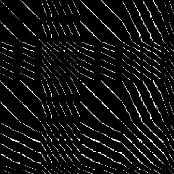
The data extracted from SUMO has information about positions, speeds, and lanes of the 3000 vehicles in the simulation. The position information can be fused with the map of the environment to obtain relative positions of vehicles conserving the traffic rules. Due to the extreme size of the dataset, spectral clustering was performed on the set of vehicle pairs that were co-present in the simulation. In a 3000 × 3000 sparce grid of cells, the cells with data were rearranged to the closest configuration to a diagonal matrix. This rearrangement of data allows for much shorter processing times when extracting data for the DBN. A visual representation of the spectral clustering can be viewed in Figure 3 and Figure 4. Each white pixel in the grid represents co-present vehicles and the black background represents empty fields. The spectral clustering rearranges the order of vehicles such that a rolling window captures the vehicle in the simulation environment. In other words, it sorts the vehicles in a quasi-chronological order in the direction of the matrix’s diagonal. This will significantly reduce the search time for co-present vehicle data and the required memory for preprocessing tasks.

The DBN topology is not guaranteed to be optimal and relies on the experts’ subjective judgement. In this case, the variables were chosen with two main objectives in mind:

1. Having the least pre-processing requirements.
2. Being the most convenient to measure from the environment in a real driving scenario.

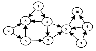
After the spectral clustering, the following variables were extracted from the dataset by fusing the position, speed, and lane data with the roundabout layout. The variables, their states, and their layout can be found under Table 1.

Table 1 DBN topology, and variables states

#	Variable Name	Variable States
1	Lane	{1,2}
2	Start Position	{E,N,W,S}
3	Entered RA[1]	{True,False}
4	Lane in RA	{1,2}
5	Destination	{E,N,W,S}
6	Inside RA	{True,False}
7	Stop to Enter	{True,False}
8	Lane Prime[2]	{1,2}
9	AccFlag[3]	{Negative, non-Negative}
10	AccFlag Prime	{Negative, non-Negative}

¹ RA stands for “Roundabout”

²“Prime” refers to the variable in the next time-slice

³ Acceleration Flag

3. 3. CVPM Implementation and DBN Interfacing

This study experiments with a variety of CVPMs to find the best one for this application. The most common sequence predictors used in this art are the vanilla RNN, GRUs and LSTMs, therefore those are the methods of choice for this study. The input and output for the three different implementations are the same and consist of a 12-second velocity history, complemented by the DBN stream. The DBN stream consists of the likelihood of one setting for binary variables, and the mean and the likelihood of the setting with maximum likelihood for non-binary variables. In this specific application, due to low number of DBN nodes, it was possible to feed all the variables into the CVPM to complement the velocity history. To keep it fair between the three methods, the number of layers and nodes were kept consistent throughout the trials, as well as training properties. One thing to keep in mind, however, is that in the case of complementary inputs, the DBN stream in this case, the closer the sequence predictor structure to a perceptron, the smoother the output and the higher the accuracy. This is validated by the results illustrated in the following figures. Also, to keep the results fair, Kalman smoothing was not implemented in these results, however, Kalman filter has shown to improve the prediction results in [14].

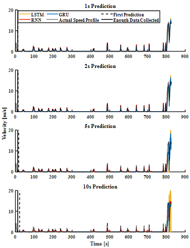
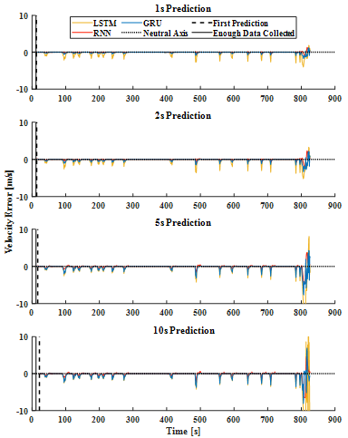
Stacked plot with the RNN, GRU and the LSTM results of heavy traffic are generated and illustrated in Figure 5, with errors in Figure 6. For having been trained with the same training parameters, LSTM with the highest number of trainable parameters yields the lowest accuracy epoch-for-epoch, which is consistent with what was expected. A better meter for scalability of these approaches can be the number of iterations per second. RNN was trained at 2.5 iterations per second, whereas GRU’s training was at 0.54 iterations per second and LSTM’s at 0.52 iterations per second. To put these figures into perspective, considering RNN as the baseline, the GRU performs 357.5% worse, while LSTM yields 380%. As a result, RNN is the most efficient CVPM of the bunch.

A look at results regardless, shows a very tight competition between the GRU’s and RNN’s accuracy for the large transient near the end where the vehicle is jetting out of the simulation environment having left the roundabout. However, the edge RNN has over the other strategies shows in prediction of the smaller movements in between the long periods of stop. As these are results of heavy traffic during the simulation (notice the large periods of stop from the beginning until second 800), these small movements are all that is available to make predictions on, and their small value should not undermine their importance.

Prediction results for a lighter traffic scenario is illustrated in Figure 7. The time this vehicle spent traversing the same length is one third of the trip in the heavy traffic scenario. As a result, the long stop periods are absent in these trips. Resultantly, the prediction strategy needs to be able to predict micromovements throughout the trip as opposed to long stops and short bursts of speed transients. The results here show a less promising performance from GRU and confirm the superiority of the RNN. Another noteworthy takeaway from examining these results is the fact that despite the fundamental differences between the behavior the motion compared to the heavy traffic results (short bursts vs consistent micromovements) the changes are reflected in the predictions which can be attributed to the DBN stream.

The DBN stream Can also be a loose explanation for why the RNN produces more accurate results than its competition. While the observed velocity history is fed as a data sequence into the CVPM, the DBN stream is held constant which is a counter to ideal working conditions of the modified RNN variants, however, vanilla RNN is insensitive to these circumstances. This however cannot be held as a fault of the approach as the solutions and workarounds would only overcomplicate the strategy,

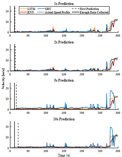
Sacrifice performance, and achieve little accuracy improvements. To have discussed the accuracy figures quantitatively, the error bounds for normal driving scenario for the RNN are [-0.71,0.94], [-0.97,1.47], [-1.46,2.75], and [-2.11,4.10], and in the case of heavy traffic driving are also measured at [-0.75,1.23], [-1.58,2.25], [-4.62,4.63], and [-6.64,6.74] m/s for 1, 2, 5, and 10 second predictions respectively. One notable item in these results is that low speed predictions are a lot more accurate than the final high-speed transients as the vehicle is jetting off the simulation environment.

Finally, the accuracy and validity of the results presented were measured by cross-correlations between actual data and the predicted speed profiles. These metrics for the RNN in the scenario presented in Figure 7 are shown in Table 2. As expected, the higher the prediction horizon, the lower the accuracy, but the results maintain a correlation greater than 0.895 and an RMSE less than 0.036.

Table 2 Accuracy metrics for RNN results of light traffic

Prediction horizon	Correlation	RMSE
1 second	0.97641	0.029334
2 seconds	0.97792	0.028453
5 seconds	0.97661	0.029249
10 seconds	0.96462	0.035995

4. Conclusion

This study proposes a versatile, real-time implementable traffic participants behaviour predictor and situational awareness strategy for roundabout driving. The results of this study can be integrated with model predictive controllers similar to the ones in [4] and [3] to improve performance and achieve autonomy in specific driving scenarios where expert data is available, and the general layout of the environment is known. Although there is no guarantee that the expert-yielded topology for the DBN is the optimal one, the one proposed in this specific use-case proved to be accurate and produced valid results for different scenarios, however, to achieve a well-rounded package that can produce accurate predictions for any roundabout, two aspects need to be improved. The hypothetical situational awareness package needs to be trained with data considering all infrastructure layouts, and needs to be able to identify the situation before generating the table of variables and their states, similar to the one in Table 1. However, that would be an extension of this very method and the principles remain the same.

Acknowledgement

The authors would like to thank Toyota, NSERC, and OCE for their generous support of this project.

References

[1] B. Sakhdari and N. L. Azad, "A Distributed Reference Governor Approach to Ecological Cooperative Adaptive Cruise Control," IEEE Transactions on Intelligent Transportation Systems, vol. 19, p. 1496–1507, 2018. View Article
[2] B. Sakhdari and N. L. Azad, "Adaptive Tube-Based Nonlinear MPC for Economic Autonomous Cruise Control of Plug-In Hybrid Electric Vehicles," IEEE Transactions on Vehicular Technology, vol. 67, p. 11390–11401, 2018. View Article
[3] S. Tajeddin, S. Ekhtiari, M. Faieghi and N. L. Azad, "Ecological Adaptive Cruise Control With Optimal Lane Selection in Connected Vehicle Environments," IEEE Transactions on Intelligent Transportation Systems, p. 1–12, 2019.
[4] M. Vajedi and N. L. Azad, "Ecological Adaptive Cruise Controller for Plug-In Hybrid Electric Vehicles Using Nonlinear Model Predictive Control," IEEE Transactions on Intelligent Transportation Systems, vol. 17, p. 113–122, 1 2016. View Article
[5] Critical Reasons for Crashes Investigated in the National Motor Vehicle Crash Causation Survey, 2015.
[6] 2015 Motor Vehicle Crashes: Overview, NHTSA’s National Center for Statistics and Analysis, 2016.
[7] D. Watzenig and M. Horn, Automated Driving Safer and More Efficient Future Driving, Springer International Publishing, 2018. View Article
[8] F. Zhang, J. Xi and R. Langari, "Real-Time Energy Management Strategy Based on Velocity Forecasts Using V2V and V2I Communications," IEEE Transactions on Intelligent Transportation Systems, vol. 18, p. 416–430, 2017 View Article
[9] C. Sun, X. Hu, S. J. Moura and F. Sun, "Velocity Predictors for Predictive Energy Management in Hybrid Electric Vehicles," IEEE Transactions on Control Systems Technology, vol. 23, p. 1197–1204, 2015. View Article
[10] E. Thorsell, "Vehicle speed-profile prediction without spatial information," 2013.
[11] J. Pearl, Bayesian networks, Computer Science Dept., University of California, 1998.
[12] Z. Ghahramani, "Learning dynamic Bayesian networks," in International School on Neural Networks, Initiated by IIASS and EMFCSC, 1997.
[13] P. A. Lopez, M. Behrisch, L. Bieker-Walz, J. Erdmann, Y.-P. Flötteröd, R. Hilbrich, L. Lücken, J. Rummel, P. Wagner and E. Wießner, "Microscopic Traffic Simulation using SUMO," in The 21st IEEE International Conference on Intelligent Transportation Systems, 2018.View Article
[14] M. Zamani Abnili and N. L. Azad, "Universal Forecasting Model for Context-Aware Perception in Autonomous Highway Merging," (Under Review).