Journal of Machine Intelligence and Data Science (JMIDS)

1. Introduction

The company to be evaluated is a SME (Small and Medium Enterprise) in the tourism sector, focused on providing high-value vacation programs or tourist packages, offering a dynamic, personalized, and innovative quality service for its client portfolio. Likewise, it began operations in 2016 and to date has firmly maintained its consolidation in the travel and tourism sector; reaching important commercial agreements with companies such as Assist Card, PlusUltra, CopaAirlines, Latam, Avianca, among others. Below is a summary of the historical data of annual sales from 2019 to 2022 as shown in table 1.

Table 1: Annual turnover.

YEAR	2019	2020	2021	2022
BILLING ($)	915 593.95	294 545.72	618 829.42	1 403 500.45

The present work of the Industrial Engineering degree addresses “Operation Research & Analysis” as a line of research for the application of mathematical modeling that allows the improvement of the sales forecasting process as support for the company's decision making.

The main objectives are to identify and determine the mathematical modeling tools to use, perform the sales forecast with the selected tools, design possible scenarios with medium-term forecasting methods, determine the size of demand, the economic impact on the company and decrease the mean absolute percentage error between sales forecasts and actual sales using the highest precision tool.

According to the research topic, the industrial engineering tools used to reduce the mean absolute percentage error between the sales forecast and actual sales are the following: Simple average, moving average and exponential smoothing. Additionally, to define the size of the sales force, the seasonal breakdown was used. With this tool, we will determine the number of average salespeople, assuming a constant level of productivity in the sales units.

2. State of the art

Regarding the technical gap, the mean absolute percentage error of companies in the tourism sector was identified as equivalent to 12.03% [1]. For its part, the company exceeds this value with 19.60% in 2022. Thus, creating a margin of opportunity to improve of 7.57%. Likewise, the quantitative analysis allowed us to calculate the economic impact caused by the absence of methods, lack of structure of the sales effort and the imbalance of data, resulting in a loss of $16 789.02.

With the help of the systematic review of the literature, it was possible to identify, evaluate and describe research articles classified according to the criteria according to their typology, as well as descriptive articles, case studies and experimental cases. Which contributed to the analysis of the tools to be used [2].

In accordance with the previous point and based on the objectives of the research, a comparative matrix will be established to define the proposals for each aspect. Two scientific articles have been selected for each tool to be evaluated. In terms of the objectives, priority is given to those that address the main reasons for the problems. Table 2 presents a comparative matrix.

Table 2: Comparative matrix and systematic literature review.

Root Causes	Engineering Tools	Scientific Article
Unstructed database	Moving average	Carolina del Pilar (2017) [3]
Inaccurancy of sales records	Simple average	Ackerman, A. & Sellito, M. (2022) [4]
Fluctuations not considered	Smoothing exponential	Marroquin, R (2018) [5]
Inadequate sales force calculation	Seasonal breakdown	Cisneros-Martinez, JD & Fernandez- Morales, A (2016) [6]
Absence of sales indicators	Seasonal breakdown

 

3. Methodology

The methodological design of the research is oriented towards process improvement. The approach is quantitative and will be based on the analysis of monthly data from closed sales, sales that have been quoted, approved, and paid for by the clients, corresponding to the years 2019, 2020, 2021, 2022, and the first quarter of 2023. It is acknowledged that the services offered by the entity in its vacation and tourism programs include transfers, accommodation, meals, guiding or advisory services, scheduled visits, and assistance cards or insurance. However, for the purpose of this study, the revenues generated by these services will be considered as a consolidated unit, allowing for a comprehensive analysis of the financial results.

The methodology is oriented to the use of machine learning using demand forecast models using the historical data of a company in the tourism sector to calculate the mean absolute percentage error of the company. In addition, the aim is to project future sales and thereby calculate the number of salespeople needed until the end of the year. Therefore, clean and filtered data is required through exploratory data analysis to use the information in the models.

The tools used are seasonal breakdown for sales force calculation while smoothing exponential, simple and moving average for demand forecasting. On the other hand, Python codes will be used to estimate the company's sales in 2024 through Google Collaboratory. Likewise, exploratory data analysis will be necessary to obtain atypical data thanks to the Orange Data Mining software, which will also allow sales for the month of September 2023 to be calculated.

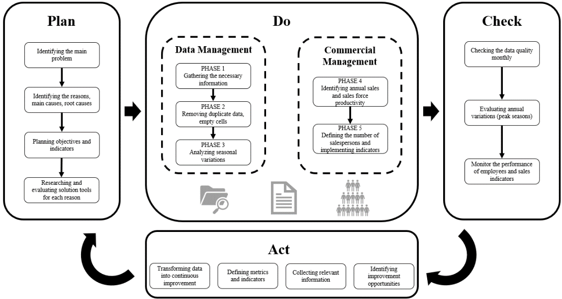
Likewise, data visualization must be used using tools such as Power Bi to analyse the results that will be delivered to the company. Below is figure 1 with the summary of the methodology.

3.1. Model components

Component 1 (Plan) To carry out the research, you must first know the company's problems and identify possible solutions. In this way, you can search for the models and tools necessary to make the improvement.

Component 2 (Do) Data management is important to ensure quality and analysis of seasonal variations in sales. The company database must be obtained that includes sales made per year with a monthly breakdown. The data was obtained from the past 4 years. The data was considered structured, since it was presented in Excel through a dynamic table with attributes such as date, seller, amount, and type of sale. Like all data, a cleaning process must be carried out to verify any problems that could lead to errors in the models such as atypical sales, duplicate data or the absence of data. In addition, the data must be consolidated with the necessary attributes, in the case of Orange and Google Collaboratory, it must include the date and annual amounts with a monthly breakdown while for the report in Power Bi, the name of the seller is also considered.

Component (Check + Act) The calculation of the forecast and the average absolute percentage error of all the years that have closed data (2019 to 2022) is carried out, each of the three selected models will be applied, which are simple, moving average and exponential smoothing. In this way, it is desired to compare and analyse the model that best fits the data, including the required seasonality. On the other hand, the data must be uploaded to Google Collaboratory so that the sales estimate for the remainder of the year 2023 and 2024 can be made. Regarding the information for the month of September, as it is a month in which the evaluation, and therefore, the data for the entire month is not available, the Orange Data Mining software must be used to predict the average value of the month. On the other hand, the data must be imported into Power Bi from the years with complete data without forecasting so that the company can observe the evolution of its sales, the scope of the sellers and the error they present to estimate their demand, which leads to the unnecessary hiring of sales force or lack thereof. In this component, the review of the previous ones is required, where, through the technical gap, the aim is to reduce the average absolute percentage error of the company. Currently, it has 19.60% while the sector average is 12.03%. For the improvement proposal, we will seek to achieve a percentage between 12 to 15 for the year 2024, so an analysis will also be carried out at the YTD (year-to-day) until the full month obtained from the Google Collaboratory estimate for the year 2024. In this way, the company will look for strategies to achieve the forecasted sales. For the sales force, with what was obtained and the calculated productivity, the number of people that must be included in the sales force to achieve the objectives will be analysed.

4. Implementation and Results

4.1. EDA technique (exploratory data analysis)

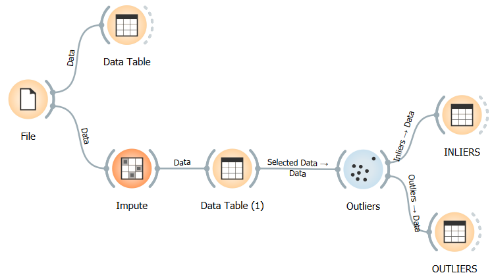
All analysis is done with Orange Data Mining software to determine atypical sales, data duplication and thereby ensure the quality of our data set. For the exploratory data analysis, the data is first displayed in the “data table” module to verify that there are no missing data. In this case, the month of September is unknown data, so with the impute module and with using the average/most frequent technique, the data for the month of September is obtained for the year 2023. The technique used in the program will be shown in figure 2.

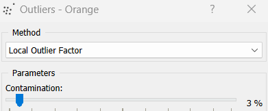
Subsequently, the table is displayed again with the data already verified in the “data table (1)”. Finally, the “outliers” module is used to verify whether there are outliers, therefore, the “local outlier factor” method is used with a contamination parameter of 3% for the minimum amount of data as we can see in the following image.

The modules used in the program are shown in figure 4.

4.2. Sales projections

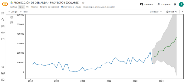
Google Collaboratory is used to project sales from October 2023 to August 2024, using Python codes, within which the 3-month seasonality due to summer vacations is considered. In figure 5, the sales trend and the projection for the year 2024 are shown.

In addition, the numerical values are presented in the following table.

Table 3: Sales projections.

Date	Forecast_Sales ($)
31/10/2023	137 409.83
30/11/2023	172 038.80
29/12/2023	161 222.12
31/01/2024	151 410.08
29/02/2024	173 791.51
29/03/2024	166 726.55
30/04/2024	159 679.85
31/05/2024	176 327.17
28/06/2024	170 047.00
31/07/2024	201 097.24
30/08/2024	138 039.88

4.3. Comparison of mathematical models

With the complete and projected annual data, the three exposed models are developed, exponential smoothing, simple and moving average in such a way that the model that best suits the needs of the company is chosen, considering seasonality and the lowest average absolute percentage error. The following table shows the summary of the results obtained from each model.

Table 4: Comparison of mathematical models.

Model (2023)	%
Smoothing Exponential	31,0%
Simple Average	23,4%
Moving Average	15,19%

As demonstrated, the moving average model will be used with a seasonality of 3 months, therefore, the calculation of the model with its respective sales and the forecast is presented.

Table 5: Comparison of mathematical models.

Year’23	Closed Sales ($)	Forecast ($)	Error (Closed Sales - Forecast)	Absolute error
			Jan		105 689.51
Feb	132 286.96
Mar	113 301.53
Apr	94 627.40	113 405.29	-18 777.89	18 777.89
May	143 742.95	117 223.96	26 518.99	26 518.99
Jun	151 485.79	129 952.05	21 533.74	21 533.74
Jul	213 187.59	169 472.11	43 715.48	43 715.48
Aug	83 556.11	149 409.83	-65 853.72	65 853.72
Sep	76 970.50	124 571.40	-47 600.90	47 600.90
Oct	137 409.83	99 312.15	38 097.68	38 097.68
Nov	172 038.80	128 806.38	43 232.42	43 232.42
Dec	161 222.12	156 890.25	4 331.87	4 331.87
		156 890.25		23 823.80

On the other hand, the analysis of the complete years from 2019 to 2023 is presented in the following table, considering the year 2020 as an atypical year due to COVID-19.

Table 6: Analysis of the complete years from 2019 to 2023.

Closed Sales (year)	Forecast ($)	Mean Absolute error	%
2019	69 676.73	11 293.96	16.21%
2020	25 987.42	19 267.51	74.14%
2021	96 178.05	17 659.53	18.36%
2022	122 828.18	24 069.87	19.60%
2023	156 890.25	23 823.80	15.19%

Finally, a calculation is carried out at YTD (January-August) of all years using the same model, focusing on the year 2024 for the projection and determining the sales of the last months to equal the mean absolute percentage error to the year 2023 (year with the lowest MAPE since 2019). The results are shown in table 7.

Table 7: YTD calculated.

Closed Sales (year)	Forecast ($)	Mean Absolute Error
2023	156 890.25	23 823.80
2024	X	19 222.93
	X = 126 591.50

The calculation of X represents the forecast that must be obtained for the months from September to December.

Table 8: Forecast from September to December.

SET-DEC	Forecast ($)	Mean Asolute error	%
Closed Sales’23	156 890.25	23 823.80	15.19%
Closed Sales’24	126 591.50	19 222.93	15.19%

4.4. Sales force calculation

Finally, by applying the sales force formula through the seasonal breakdown model, we obtain the number of workers required for the year 2023. The example is presented in Eq. 1 as follows:

(1)

(2)

(3)

N is obtained, which represents the number of workers.

4.5. Data visualization

Power Bi software is used to view the general report that includes sales by year and month, the necessary sales force and the results and indicators that have been previously evaluated. The following figure shows the main page.

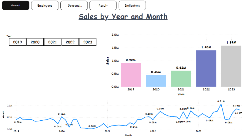
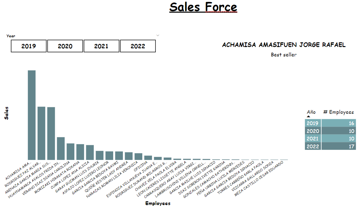
5. Discussion and Results

The design of the initial proposal based on the systematic literature review, it allowed us to identify and select the necessary industrial engineering tools to build the demand forecasting model [7]. Likewise, to decrease the mean absolute error between the sales forecast and the actual sales. The choice of the appropriate tool will depend on the behavioral pattern or trend of historical data in demand, also determined by their seasonality. Smoothing exponential is another tool that proposes an improvement in terms of forecasts, since, as time passes, each period decreases its weight. 7 different models were compared, among which the moving average, weighted moving average, exponential smoothing, holts, winters, and direction stand out; However, for the proposal of an inventory management system based on demand forecasts and the minimization of the MAPE error, the forecasting methodology with the lowest error is single smoothing exponential [5]. Based on historical sales data, a model is sought to help anticipate the demand that the company will receive. Demand estimation models for pellets for home use, industrial use and proposed process and information management for demand forecasting [8].

This research aims to identify and select the necessary industrial engineering tools to build a more accurate demand forecasting model, specifically focused on the tourism sector, with the goal of reducing the current mean absolute percentage error (MAPE) from 19.60% to a target of 12.03%. Improving the accuracy of the forecast will optimize the company's strategic decisions by providing a more reliable analysis of future demand [9]. To achieve this, various tools such as simple averages, moving averages, and exponential smoothing were considered to evaluate which one is most effective for the company in question. The research also integrated advanced approaches like machine learning and predictive analysis, using Orange Data Mining for exploratory data analysis, Python in Google Collaboratory for sales estimation, and Power BI for result visualization through interactive dashboards that facilitate management decision-making. As for the results, sales were estimated for the remaining months of 2023 and some of 2024 using these forecasting tools and techniques. Additionally, seasonal decomposition allowed for an accurate calculation of the number of workers needed, which helps in better human resource planning and reduces the likelihood of operational inefficiencies [10]. These projections, beyond improving the accuracy of demand forecasting, have economic, social, and environmental implications [11]. From an economic standpoint, reducing the MAPE optimizes inventory management, which not only reduces costs associated with stock management but also frees up capital that can be reinvested in commercial strategies, plant expansion, or the inclusion of new products in the portfolio [12]. From a social perspective, an improvement in forecast accuracy increases customer satisfaction by ensuring the availability of products or services at the right time, which enhances the company’s competitiveness and its position in the market, helping it to reach "Top of Mind" status [13]. Environmentally, an increase in sales due to better planning could encourage companies to adopt more sustainable practices, thereby contributing to environmental conservation.

Regarding the discussion of results, the use of the moving average stood out as one of the most effective tools. This technique, based on the arithmetic mean of historical data, is used to forecast the next period and is particularly useful when demand is stable and shows no trends or seasonality. In this research, a set of historical observations was used, which allowed for precise analysis of demand over time [14]. On the other hand, weighted averages were implemented for cases where data did not have the same relevance, allowing forecasts to be better adjusted to the company’s reality. Methods such as the moving average and exponential smoothing, which included an alpha of 0.7, proved effective for producing quick, cost-effective, and accurate forecasts, especially in medium-term scenarios by giving more weight to the most recent information in the time series. Compared to other studies, such as Vernaza’s application of similar tools to forecast demand in a printing company, or the case of MASONITE, a door manufacturer, this research revealed that using exponential smoothing with an alpha of 0.7 was effective in reducing MAPE for several products, although the moving average also yielded results very close in terms of accuracy [15].

In this investigation, tools like Microsoft Excel Solver were used to optimize the calculations for exponential smoothing with an alpha of 0.4 and for calculating moving averages with a period of 3 months. The results showed that the moving average was the most convenient tool for demand projection, achieving a MAPE of 28.73%. On an economic level, the results were equally positive, with a Net Present Value (NPV) of $ 7 565.98, indicating that the investment is recommended since the NPV is above 0. Furthermore, the internal rate of return (IRR) of 26% is higher than the cost of capital (COK) calculated at 15%, reinforcing the viability of the project. The benefit-to-cost ratio of 2.60 is also greater than one, indicating that the benefits significantly exceed the costs involved.

Google Collaboratory projections and the moving average tool were used to reduce the mean absolute percentage error for the year 2023, achieving a rate of 15,36%, whereas in the tourism sector, it stands at 12,03%. Nevertheless, there was a 4,24% reduction in MAPE compared to the year 2022. To compare scenarios, a table will be created with key indicators for each.

Table 9: Economic indicators of the improvement project.

Criteria	Normal	Optimistic
MAPE	15.36%	12.03%
Economic NPV	$7 422.58	$7 961.64
Economic IRR	26%	27%
Benefit / Cost	2.58	2.70
Recovery period	3 months and 5 days	3 months and 12 days

All scenarios show positive NPV (Net Present Value), IRR (Internal Rate of Return) and Benefit/Cost, but the key difference is in the Benefit, as the project aims to boost income by reducing the mean absolute error.

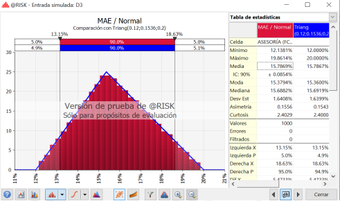
Risk will be used to define both input and output variables. First, the variables to be calculated must be defined. In this case, the main indicator is the MAPE, and the simulation will be based on this input indicator with its respective scenarios. Regarding the distribution, the triangular distribution will be selected due to three scenarios, as mentioned earlier, including a pessimistic one considering a 20%. This is shown in table 10.

Table 10: Criteria for Risk Simulator

Criteria	Pessimistic	Normal	Optimistic
MAPE	20%	15.36%	12.03%

The average MAPE in the simulation was 15.7867%. However, in the project improvement, it was 15.36%. This means that the project improvement, along with the tools used, is feasible to achieve a lower MAPE, thereby increasing income by estimating an adequate demand. The simulation is shown in Figure 8.

6. Conclusion

The research concludes that applying quantitative methods such as moving averages, exponential smoothing, and technological tools like Python and Power BI, combined with simulations in Risk Simulator, provides a robust solution for demand forecasting in tourism sector companies. Although the target of a 12.03% MAPE was not achieved, an error of 15.36% was reached, indicating significant improvement in forecast accuracy. The Risk Simulator simulation validated the results with a MAPE of 15.78%. Additionally, the systematic literature review compared this work with previous studies, showing that optimal tool selection depends on historical data behavior and demand seasonality. In summary, this work improves demand forecasting accuracy and positively impacts competitiveness, customer satisfaction, and operational efficiency, highlighting the importance of adopting advanced technologies and quantitative methods to maintain a competitive market position.

Companies must adapt to technological advancements by implementing tools and strategies to maintain competitiveness and drive growth. In this improvement project, a tool was developed to calculate the Mean Absolute Percentage Error (MAPE) of sales, accounting for seasonal variations through annual rest periods. Data from previous years was supplemented for 2023 using Python in Google Collaboratory, allowing for sales forecasts to be made before year-end and optimizing MAPE calculations. Various techniques were employed, including exponential smoothing, moving and simple averages. The moving average method proved to be the most effective, resulting in a 15.36% error. In the tourism sector, the average MAPE is 12.03%. Although this project recorded a MAPE of 15.36%, it achieved a 4.24% reduction compared to the previous year. Additionally, a sales team of 20 employees was anticipated by 2023; however, only 15 were reached by August. Analysis with Risk Simulator confirmed the effectiveness of the tool and Python for forecasting, generating a Net Present Value (NPV) of $7,422.58 with a MAPE of 15.36%.

References

[1] Díaz, F. R., & Romaní, Y. L. (2022). Universidad del Zulia. View Article
[2] Pérez, A., Cruz de los Ángeles, J., Guatemala, A., & Juárez, V. (2018). Importancia de los pronósticos en la toma de decisiones en las MIPYMES. Revista GEON (Gestión, Organizaciones Y Negocios). View Article
[3] Sánchez Sepúlveda, Carolina del Pilar (2018). Medición en la precisión de los pronósticos de ventas y su efecto en los costos de la empresa. Universidad Andres Bello View Article
[4] Ackermann, A. & Sellito, M. (2022). Métodos de pronóstico de la demanda: una revisión de la literatura. Revista Innovar. View Article
[5] Marroquín, R. (2018). Propuesta de un sistema de gestión de inventarios a partir de pronósticos de la demanda dentro de una imprenta (Tesis de pregrado). Universidad de las Américas, Quito. View Article
[6] Cisneros-Martínez, J, & Fernández-Morales, A. (2016). Concentración estacional de la demanda hotelera en Argentina. Revista de Estudios Regionales.
[7] López, A. (2018). Establecimiento de KPI y generación de predicción de la demanda para el grupo "viajar por escocia" (Tesis de Máster). Universidad de Valladolid. View Article
[8] Ibarra Salazar, J., & Sotres Cervantes, L. (2005). Estimación de la demanda de viajes en el aeropuerto de Querétaro. ProQuest. View Article
[9] Castro, J. (2021). Modelo de pronósticos. Repositorio de la Universidad Técnica del Norte. View Article
[10] Colther, C., & Arriagada-Millaman, A. (2021). Pronóstico de la demanda turística de Chile basado en modelos lineales y no lineales estacionales. Revista de Turismo y Patrimonio Cultural. https://doi.org/10.25145/j.pasos.2021.19.021 View Article
[11] Ruíz, H. (2018). Pronóstico de las exportaciones del cacao ecuatoriano para el 2018 con el uso de modelos de series de tiempo. UIDE.. https://doi.org/10.33890/innova.v3.n6.2018.713 Saeteros, A., & Vicente, E. (2017). Análisis de la Demanda del Turismo para la Gestión Sustentable del Destino en las Islas Galápagos-Ecuador. ABET. View Article
[12] Contreras, A., Zuñiga, C., Martínez, J., & Sánchez, D. (2016). Análisis de series de tiempo en el pronóstico de la demanda de almacenamiento de productos perecedero. Elsevier España. http://dx.doi.org/10.1016/j.estger.2016.11.002 View Article
[13] Coto-Solano, M. (2018). Estimación de Demanda de Tránsito: modelos clásicas, basado en circuitos y basado en actividades. (Revisión Literaria). Tecnología en Marcha. https://doi.org/10.18845/tm.v32i2.4353 Díaz-Pinzón, J. (2020). Precisión del pronóstico de la propagación del COVID-19 en Colombia. Revista Repertorio de Medicina Y Cirugía. View Article
[14] González, B., Hernández, Y., & Rodríguez, M. (2021). Propuesta metodológica de diagnóstico de los sistemas de distribución comercial en las agencias de viajes. Revista Internacional de Turismo, Empresa y Territorio. https://doi.org/10.21071/riturem.v5i1.13426 View Article
[15] Gónzalez, L. (2022). Diseño de modelo de pronóstico de demanda de ventas para la empresa más moda PET [Tesis de licenciatura, Universidad Pascual Bravo]. Repositorio de la Institución Universitaria Pascual Bravo. View Article