Journal of Machine Intelligence and Data Science (JMIDS)

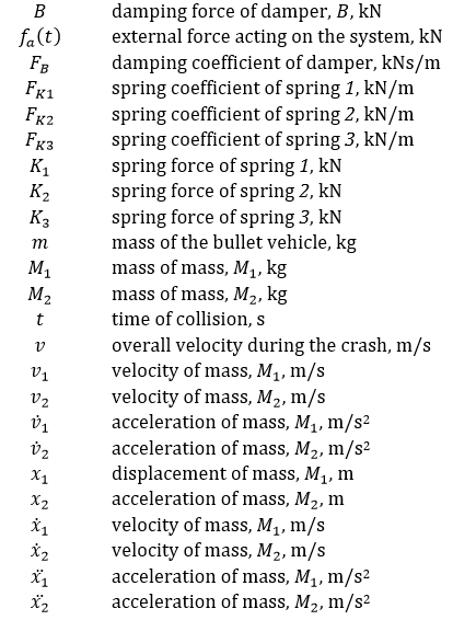
Nomenclature

1. Introduction

Automobile accidents are very unpredictable and can happen in a multitude of different ways, with an infinite number of factors and contributors, making them one of the harder circumstances to study and analyze. This is why it is essential to have many differing forms of tests and models to learn about the behavior of not only the vehicles involved in the crash, but also the critical components that comprise each vehicle.

There are many previous works aimed at establishing reliable mathematical models for vehicle collisions using various types of analytical simulations. Specifically, the work performed in [1] describes the process of using Newtonian Mechanics to obtain a table of results that illustrates the properties of two vehicles during a two-dimensional collision. This research focuses on the vehicles as objects, determining how the properties of the entire vehicle will behave before, during, and immediately after a crash. However, in the simulation and analysis discussed in our paper, the components in front of the sedan’s firewall were included in the scope of work because the front bumper assembly, engine, and engine components can displace greatly during a frontal crash. This often causes expensive and sometimes irreparable damage to the vehicle. The engine components being considered in this study are items such as the transmission, camshaft, and similar items connected directly to the engine block. These were taken to be mass M₁. The front crash bar, bumper, and front body paneling were taken to be M₂. The displacements of these masses were the main points of interest during the simulation.

Mathematical models can also be used to model collisions between a vehicle and a stationary object, such as a bridge pillar, as explained in [2]. By analyzing one moving object and one stationary object, some simplification of the mathematical model may be performed, in order to focus on specific results, or in this case, focus on a new type of force model. Our study considers two separate vehicles involved in the collision, one being the vehicle that was considered the bullet vehicle (faster vehicle), and the other being the target vehicle, which was moving at a much slower speed. According to the National Safety Council, approximately 70 percent of automobile accidents involve multiple vehicles, rather than one vehicle and a stationary object [3]. This is the main reason two vehicles were considered, rather than just a single vehicle colliding with a stationary object such as a tree. The bullet vehicle was taken to be a 2007 Audi A4 sedan with a mass of 1,600 kilograms. This specific vehicle was used because it is a vehicle that the author is familiar with and understands how the vehicle behaves during a frontal crash. The target vehicle was a much larger vehicle, like a truck, and its slower speed was added to the speed of the bullet vehicle to determine the total force acting upon the Audi’s component system. Another purpose of this simplification is that the speed of the bullet vehicle was much faster than that of the target vehicle (8 m/s to 2 m/s), and by adding the speeds together, the calculation of the force would be more straightforward for the entire system.

Another variable that the crash simulation in this paper considers is the effect of subzero temperatures on the friction coefficient of the road surface, which plays a vital role in both the “pre-impact” and “post-impact” stages of the collision [4]. This variable changes both how the car behaves when the brakes are applied before impact, and how the vehicles displace after the crash. Combining these factors with those listed above makes this dynamic collision model very unique.

Collision Model

In order to obtain an accurate result for the two governing equations that were formulated for this system, a proper diagram of the system needed to be created showing the masses, springs, dampers, and any stationary objects within the system. This model is shown below in figure 1.

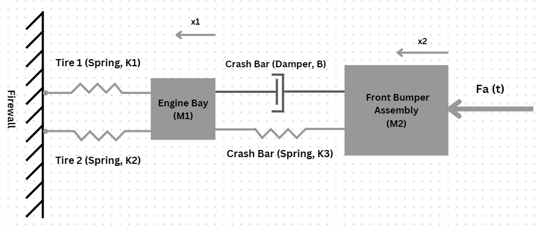
Looking at the figure, it can be seen that there are two different masses within the system, each with their own respective displacements x₁ and x₂. Mass M₁ is attached to the stationary firewall of the vehicle by the two tires that are modeled as springs in this system (more on this later). The tires on the Audi A4 are located slightly behind the engine, so it is acceptable to take them as the connecting component between the engine and the firewall for the sake of simplicity. The mass M₁ is connected to mass M₂ by the supports located between the crash bar and the engine. These supports are made of mostly aluminum and a small amount of steel, so they can be modeled as both a spring and a damper due to aluminum being a highly ductile material. The final force that is acting within the system is the input force from the actual collision between the two vehicles. Because this was a frontal crash, the crash bar, M₂, is the mass that is directly affected by force caused by the collision.

2.1. Forces Within the System

Each of the individual components contained within the system exhibit their own forces on other objects in the system besides the masses M₁ and M₂. This is because the masses are what the forces act on and do not have their own source of force. Using figure 1, it can be speculated that the displacement of mass M₂ will be greater than the displacement of mass M₁ because the outside force is acting directly on mass M₂. The stiffness coefficient equations are all similar but use different displacements depending on which of the masses they are connected to. These are shown below as equations 1 through 3.

(1)

(2)

(3)

The damping coefficient of the damper is given below in equation 4. It is important to note that the damping coefficient uses the velocity of the masses, not the displacement, as the previous spring modelling equations had.

(4)

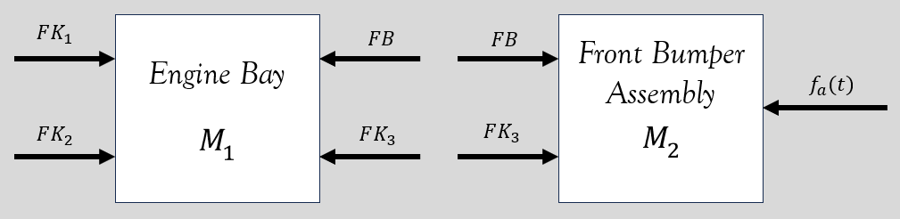
2.2. Free Body Diagram

Free body diagrams are commonly used when modelling dynamic systems to display how forces act on objects within the system using blocks and arrows. The two objects of interest within this system are M₁ and M₂ which are shown as blocks in figure 2. The forces that are acting on them come from the external force during the collision and the spring and damping forces from the other components of the vehicle. Figure 2 shows the free body diagram of the system with all forces included.

3. Dynamics

After modeling the system using the free body diagram, the direction of each force was determined, allowing for the formulation of modeling equations that represent each mass element, M₁ and M₂, respectively. The equation relating to mass M₁ is shown below as equation 5, and the equation relating to mass M₂ is shown as equation 6.

(5)

(6)

3.1. State Variable Equations

The state variables are determined from equations 5 and 6 above, looking at the masses, M, and the springs, K. Masses have variable values of velocity(), while springs have values of displacement (x₁, x₂). Therefore, in this system, between the two masses and three springs, the state variables are x₁, x₂,v₁, and v₂. Next, these state variables needed to be combined into state variable equations. This is done by taking the derivative of each of the four state variables above. For x₁ and x₂, the state variable equations are very simple. Taking the derivative of each displacement leads to the velocities of the masses as shown below in equations 7 and 8.

(7)

(8)

The process to obtain the derivatives of v₁ and v₂ is slightly more complex. The modeling equations 5 and 6 need to be manipulated in order to calculate and , which are equal to and , and are shown below as equations 9 and 10.

=

(9)

=

(10)

It is also possible to obtain a matrix relation for the state variable equations 7 through 10, and it is shown in equation 11. These matrices make it much easier to enter the equations into a computing software such as Matlab and utilize them in plots or for other coding, which is what was done to obtain the plots and results that are shown later in this research.

(11)

3.2. Magnitudes of Component Forces

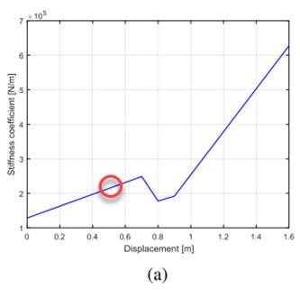
In order to utilize the matrix shown in equation 11 within the Matlab software, the magnitudes of each force variable (F_K1,F_K2,F_K2,F_B,M₁,M₂, and the external force f_a(t)) needed to be determined. The first set of forces (F_K1 and F_K2) are the tires on the Audi A4. These tires are made of rubber, so they behave as springs when any outside force is applied to them, whether it be horizontal or vertical. The tires were both of the same compound, size, and brand, so their stiffness coefficients were assumed to be the same at a value of 475 KN/m, which is a value from Advanced Tire Mechanics, and was determined using the proper tire size (225/45/R17) [5]. The final spring within the system has a stiffness coefficient of F_K3, which is labeled as the crash bar of the vehicle. The crash bar on the Audi A4 is made of aluminum and boasts properties similar to that of a spring in order to prevent deformation during a low-speed crash. To obtain the stiffness coefficient that the crash bar exerts on the system, figure 3 was used. The plot shows the relationship of the stiffness coefficient of the front bumper to displacement during an automobile crash. The circle shows which value was used in this simulation, 215 kN/m [6].

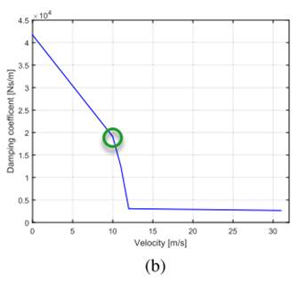
The singular damper within the system has a damping coefficient with a magnitude of F_B. There is very little data involving the use of metals as dampers, but after thorough research, it was determined that a damping force for the whole front end of the car would be used, which had been calculated during a previous study of a crash using computer software [6]. Figure 4 shows the resulting plot of the damping coefficient in kNs/m in relation to the velocity of the vehicle during the crash. Using the value mentioned in the introduction of this paper, 10 meters per second, the damping coefficient was taken to be 18.5 kNs/m.

Next, the two masses, M₁ and M₂ were to be determined. Mass M₁ was referred to as the mass of the engine bay, which means that it is the sum of the engine components within the Audi A4. The engine, transmission, and similar engine related components were all considered within this mass. By adding the mass of these components together, this value was determined to be 550 kg and was larger than the mass M₂. For mass M₂, the mass of the entire front end of the car (crash bar, bumper, quarter panels, and radiator) was determined using a simple ratio for all-wheel drive cars. Most all-wheel drive cars have a 60/40 ratio, meaning that 60 percent of the overall mass of the car is contained in the front of the vehicle, supported by the front axles. Because the total mass of the 2007 Audi A4 was close to 1600 kg, using the 60/40 rule, as well as excluding the mass that was already taken as mass M₁, the mass M₂ was approximated as 410 kg [7].

3.3. Magnitude of the External Force

The last, and arguably most important force that needed to be determined was the external force from the two vehicles colliding. This force was labeled as f_a(t) and was calculated using equation 12, then subtracting the total braking force of the front and rear brakes to simulate the brakes locking up on the vehicle, which is the case right before most crashes.

(12)

Using equation 12, the overall force due to the two vehicles colliding was calculated to be 64 kN. Now, it was important to subtract the total braking force for an AWD car. This was done using figure 5, along with the friction coefficient of pavement during near freezing conditions. As mentioned in the introduction, the crash being modelled occurred on a snowy night at near freezing temperatures. From a chart located in [8], rubber (the tires) in contact with wet snow have a friction coefficient between 0.30 and 0.60. For the sake of this experiment, and because the snow had been on the road for a substantial amount of time at near freezing temperatures, a friction coefficient on the lower side of the range was used.

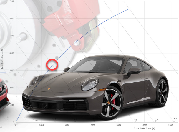
This value was taken to be 0.4 and was then used in figure 5, which shows the relationship between braking force and friction coefficient using a concept known as the “Ideal Brake Curve” [9].

In figure 5, the x-axis is the front braking force, and the y-axis is the rear braking force. By summing these two forces, the total braking force could be determined. The point of intersection along the line with a friction coefficient of 0.4 is marked with a red circle within the figure. The total braking force was determined to be 6.5 kN, and when subtracted from the total impact force of 64 N, the force f_a(t) was found to be 57.5 kN.

3.4. Modelling the System in Matlab Simulink

Matlab was the primary program used for the coding and plotting portion of this collision analysis. The Matlab sub-program, Simulink, was used in conjunction for the modelling portion of the analysis. The Simulink model for this system is shown below in figure 6.

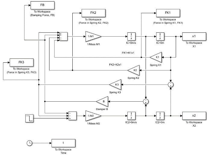
This model makes it much easier to create plots of individual forces over a specified time period because the plot commands are specified within the Matlab code, and the code can grab values from the Simulink model for each increment of time that the code is running. The Simulink model represents the same system as shown in figure 1, just displayed and connected in a way that the program can more efficiently interpret.

4. Simulation Results and Discussion

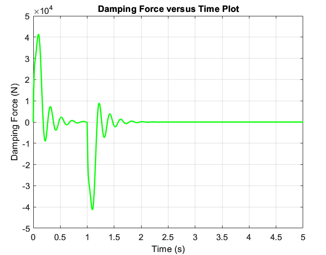
After the code was finalized in Matlab, and the Simulink model was created and properly linked to this code, the program was executed and produced the diagrams and results shown in figures 7, 8, and 9 below.

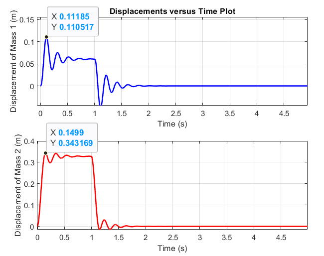
Comparing the displacements of M₁ and M₁ shown in figure 7, it can be seen that the maximum displacement of M₁ is much greater than that of M₁. This aligns with what was expected because mass M₁ has the external force f_a(t) acting directly on it, with no springs or dampers in between, unlike mass M₁, which has a spring and damper between it and mass M₂. K₁ and K₂ apply such a large spring force during the simulation that it prevents a large amount of displacement on the engine bay, M₁ as well. The fact that the springs are not directly attached to the front of the car causes the external force to act more aggressively on M₂, contributing to its larger displacement. Because of the larger displacement of mass M₂ seen within the simulation, it is expected that the front components of the vehicle would be pushed back into the engine, causing damage. This is exactly how the front portion of the bullet vehicle behaved when the author was involved in a similar crash. The front bumper components were pushed into the front of the engine during the collision, causing the timing belt to jump, locking up the engine, leading to the vehicle being unrepairable.

It would be interesting to conduct a follow up study that remodels the system, so the tires (springs) are shown as connected to the front crash bar to see if it makes a large difference on the displacement and oscillation of the two masses. Adding more components and making the model more complex will also lead to a rework of the simulation, and most likely make it more accurate. One other unique characteristic of the displacement plot is that the oscillation of mass M₁ is larger than that of mass M₂. This is also attributed to the springs K₁ and K₂. Their large stiffness coefficients resist initial displacement, but once moved, tend to oscillate for a longer period due to the small magnitude of the damping coefficient within the system.

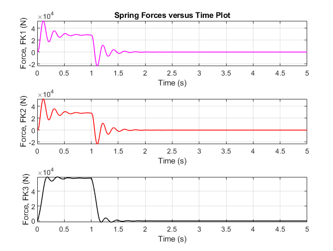
The plot of the three spring forces, K₁, K₂, and K₃ in figure 8, shows that they also have some oscillation, very similar to that of their associated displacements. The oscillation for springs 1 and 2 is larger than that of spring 3, due to the fact that their stiffness coefficients are both much larger than spring 3, so they absorb more of the energy from the crash. This means that they will oscillate more aggressively after the force is removed in relation to spring 3 that only oscillates slightly after the force from the crash is removed from the system. When the plots of springs 1 and 2 are compared, it can be seen that they are identical. This is because both of these springs have the exact same spring coefficients, and act on the same components within the system. This is a good indicator that the Simulink model was able to precisely represent the system as it was originally modelled in the free body diagram. If either of the two plots varied from one another, it would be obvious that there was an error within the code, or Simulink model. Another interesting part of the spring plots in figure 8 is that both springs 1 and 2 apply negative forces for a short time during the simulation. This was caused by the force of the crash being so large that when the springs rebounded after the initial oscillation, they were stretched by the oscillation of the masses and exerted a negative force on the masses in order to return to their original “zero” state.

The final plot that was generated from this collision simulation is shown in figure 9 and displays the damping force versus time for the duration of the simulation. This plot behaves the typical way that a damper should, beginning with a large amount of oscillation, but quickly steadying out to a damping force of zero newtons. The damper also copies the behavior of springs 1 and 2 by oscillating a large amount as the force is applied, then switching and oscillating at a much lower value after the force is removed. This behavior matches what was originally anticipated because it proves that the damper is fulfilling its purpose in helping reduce the oscillation within the springs between masses M₁ and M₂. Although the damper does not directly act on spring 3, it is able to slow down its oscillation as well because as the velocity of mass M₂ decreases due to the damping force, the force of spring 3 must also decrease in order to reach a “zero state.” It is also important to note that the maximum damping force on the system matches what was expected because it falls slightly below that of the three springs (41.5 kN) but is large enough that it is able to efficiently stop the motion of the springs, as well as the displacement of the masses.

5. Conclusion

This research illustrates a unique type of crash test, one considering a vehicle and its components at near freezing temperatures, as well as roads with reduced friction conditions. With this combination of variables, this simulation becomes a unique starting point for anyone looking to analyze a crash outside of typical parameters. By introducing new variables and different types of models into the collision dynamic system, more accurate, in depth, or situation specific results can be obtained using the already written, precise code and model within Matlab and Simulink. Future work would include modifying the dynamic analysis model, and in turn, the associated equations to obtain more accurate results.

References

[1] Beulah, G.K., Uday, B.N., “Dynamics Model of Vehicle in Two-Dimensional Collision,” Complexity International Journal (CIJ), vol. 24, no. 1, 2020
[2] Do, T.V., Pham, T.M., Hao, H. “Dynamic responses and failure modes of bridge columns under vehicle collision,” Engineering Structures, vol 156, pp. 243-259, 2018
[3] National Security Council (2023). Injury Facts: Type of Crash [Online]. Available: View Article
[4] Zhang, X., Jin, X., Qi, W., Guo, Y., “Vehicle crash accident reconstruction based on the analysis 3D deformation of the auto-body,” Advances in Engineering Software, vol. 39, no. 6, pp. 459-465, 2008
[5] Nakajima, Y. (2019). Spring Properties of Tires. In: Advanced Tire Mechanics. Springer, Singapore. View Article
[6] Munyazikwiye B., Karimi H., Robbersmyr K.G. (2017) Optimization of Vehicle-to-Vehicle Frontal Crash Model Based on Measured Data Using Genetic Algorithm [Online]. Available: View Article
[7] Auto123.com (2023) Technical Specifications: 2007 Audi A4 2.0T Quattro [Online]. Available: View Article
[8] Baker, J.S., Traffic Accident Investigation Manual, Northwestern University, Evanston, 1975, p. 210
[9] Mees H. (2023) The ‘Ideal Brake Curve’ And Why Cars Have Such Vastly Different Brake Sizes [Online]. Available: View Article