Journal of Machine Intelligence and Data Science (JMIDS)

1. Introduction

In today’s business landscape, companies compete in a market that demands high-quality products delivered as quickly as possible and at competitive prices. To be efficient in these terms, it is crucial for companies to have a well-structured and reliable production planning and scheduling function. One of the most important Key Performance Indicators (KPIs) that companies consider in this area is undoubtedly the Production Lead Time (PLT), as an accurate forecast of this indicator enables more precise and efficient production planning, allowing for a reliable prediction of the customer’s waiting time.

Moreover, having a reliable forecast of PLT is fundamental nowadays: indeed, the issue of an inaccurate prediction could have highly adverse effects on the company. Indeed, for example, if the PLT is underestimated, the inaccurate prediction leads to actual delays that might propagate throughout the entire supply chain, all the way to the end customer, who could feel disappointed or neglected, resulting in a decreased brand loyalty. However, underestimating PLT can also pose serious consequences for the company. For instance, if the time required to produce an item is less than initially predicted, the costs of warehousing the work in progress would significantly escalate.

With the advent of Industry 4.0, advanced artificial intelligence technologies are becoming increasingly relevant and utilized within the planning and production scheduling process, as they allow accurate and precise estimation of the PLT.

In this work, we aim to introduce a novel prediction process that combines supervised and unsupervised Machine Learning (ML) algorithms. Specifically, fuzzy C-medoids clustering algorithm is used as pre-processing method before the adoption of a predictive model to enhance predictive accuracy.

Clustering is an unsupervised ML model, used to partition data into homogeneous groups based on a set of segmentation variables. Among the various clustering variants, two primary approaches emerge: crisp clustering and fuzzy clustering. These two approaches differ in their ability to handle uncertainty and flexibility in point-to-cluster assignments: in crisp clustering, each data point is exclusively assigned to a single cluster, while in fuzzy clustering data points can partially belongs to multiple clusters, introducing a degree of membership that reflects data uncertainty.

Furthermore, both crisp and fuzzy clustering can yield virtual or real units as representatives of the final clusters. These two algorithms are known as C-means and C-medoids, respectively. In the C-means algorithms, the representatives are referred to as centroids and they are computed as the average of all data points within the clusters. On the other hand, in C-medoids algorithms, the representatives are referred to as prototypes or medoids and they are actual data point within the cluster selected to minimize the within-cluster distances while maximizing the between-cluster distances.

Indeed, we applied this methodology in a real case-study in which our goal was to predict the PLT for a company operating in the fashion industry: the final aim was to provide the company with more accurate predictions, allowing them to be more efficient in the planning and scheduling of the production.

This paper is structured as follows: Section 2 illustrates some related works, regarding both PLT predictions in an industrial context using ML models and the implementation of clustering as a pre-processing method for predictive models.

Section 3 presents the methodology that we propose to introduce, Section 4 provides the formal statement of the case study. In section 5 there will be a brief discussion of the findings of this case study, while Section 6 comprises the conclusions and an outline of the future work we intend to pursue.

2. Imprecise and dependent information: the case of the tourism sector

The economic impact of tourism flows is often essential for those regions/local communities in which tourism is considered the major source of income [1]. To improve the economic effects of tourism visits, appropriate data and tools are needed to study the determinants of tourism expenditure and to analyse the tourists’ spending behaviour in depth.

Section 3 presents the methodology that we propose to introduce, Section 4 provides the formal statement of the case study. In section 5 there will be a brief discussion of the findings of this case study, while Section 6 comprises the conclusions and an outline of the future work we intend to pursue.

2. Literature review

2. 1. Lead time prediction using Machine Learning algorithms

As previously mentioned in the previous section, PLT stands as one of the most crucial KPIs for a company: indeed, many production planning and scheduling methods rely on this parameter and on its forecast’s accuracy. Estimating this parameter, however, is a highly intricate endeavour due to the complexity of production processes and the wide range of products requested by the market; this phenomenon is further exacerbated by the advent of mass customization.

As stated, the goal of our study is to predict the PLT for a company operating in the fashion industry. To achieve this, we intend to leverage ML methods. Naturally, existing literature contains numerous cases regarding the forecast of Lead Time (LT) or Cycle Time (CT) using these techniques. During our literature review, we encountered numerous contributions that focus on employing ML models to predict LT or CT, but two key points, which merit significant emphasis, should be underlined: firstly, it can be asserted that there are numerous contributions investigating LT prediction using ML models in the semiconductor industry, where this KPI is absolutely critical [1]–[5].

During our literature review, we encountered numerous contributions that focus on employing ML models to predict LT or CT, but two key points, which merit significant emphasis, should be underlined: firstly, it can be asserted that there are numerous contributions investigating LT prediction using ML models in the semiconductor industry, where this KPI is absolutely critical [1]–[5].

Furthermore, an additional trend we observed is related to the presence of simulations used to test methods used for forecasting this metric. In fact, multiple examples [6]–[9], use discrete event simulations for this purpose.

A significant contribution for our study is the one presented by Rizzuto et al. [10], in which they compared various ML models to determine the most accurate in predicting LT in a drilling factory. In this work, four different families of ML models: Linear Models, Ensemble Tree methods, Gradient-Boosted Decision Trees, and Neural Networks were compared to identify the most favourable approach for delivering a precise estimate of the duration of a drilling process.

From the results of their analysis, it is possible to state that tree-based methods outperformed the other tested methodologies.

Another very intriguing contribution is the one of Lingitz et al. [1], in which various ML methods for predicting LT were compared. Here, the input data for the various models were obtained directly from the Manufacturing Execution System (MES).

In their work, Linear Models, Artificial Neural Networks, multivariate adaptive regression (MARS), Support Vector Machines (SVM) and tree-based models were compared.

Five different metrics were used to evaluate the performance of the different methods: mean absolute error (MAE), mean absolute percentage error (MAPE), mean squared error (MSE), root mean squared error (RMSE) and normalized root mean squared error (NRMSE).

As in the work of Rizzuto et Al. [10], also in this study the most performing method resulted the random forest.

Further confirmation of the predictive accuracy of Random Forest in these particular situations is provided by the study conducted by Pfeiffer et al. [6], where a factory simulation was developed and three different ML models were tested: Random Forest, linear regression, and tree based model. Once again, the top-performing model was indeed the Random Forest.

To summarize, we can affirm that there are several studies that have addressed the issue of LT prediction. We have briefly analysed three contributions, which represent the most significant ones from our perspective. From all three of these works, it has emerged that the best ML model in terms of predictive accuracy is the Random Forest.

2. 2. Cluster-based prediction

As previously mentioned in the first section, the main idea discussed in this paper is to suggest a methodology that can integrate clustering as a pre-processing method for predictive models. We have thus conducted a literature review on this topic, and one of the earliest examples we found is the work of Ari and Guvenir [11], that introduced the concept of a cluster-based linear regression algorithm in 2002. From their analysis, it becomes evident that performing clustering before applying linear regression can indeed enhance predictive accuracy.

Another highly significant contribution to this field is the work of Trivedi et al. [12], in which the idea that clustering can help in reducing errors in various prediction tasks was investigated. The methodology that they propose involves is based on three main steps: the first one is the clustering the dataset. Then, the subsequent one consists of training a predictor separately for each cluster. The predictions obtained from each predictor are then combined using a naïve ensemble. Specifically, the procedure outlined in the paper employs the use of K-means clustering algorithms in combination with three different predictive models: linear regression, stepwise linear regression, and Random Forests. The results they obtained indicate that in most of the investigated datasets, the use of clustering before applying predictive models leads to improvements, especially in the case of linear regression and stepwise linear regression. On the other hand, when this methodology is applied in conjunction with Random Forest, improvements seem relate to the size of the dataset, as in small dataset there aren’t statistically significant differences, while in bigger ones it seems that this methodology can improve prediction accuracy significantly.

In our work, we aim to implement the fuzzy C-medoids [13] clustering algorithm. This clustering algorithm differs from crisp clustering because, as already mentioned in the Section 1, while the latter assigns observations to clusters in a hard manner, fuzzy C-medoids provides the degree of membership of each observation to belong to each of the created clusters. A relevant study in the literature is provided by Nagwani et al., [14], who explored the use of clustering techniques, both crisp and fuzzy, in conjunction with regression techniques to understand if this approach would improve the predictive accuracy, when predicting the compressive strength of concrete. Their work revealed that the combined use of clustering and regression techniques minimizes predictive errors, and that fuzzy algorithms outperform crisp algorithms.

However, it’s important to note that in this study, the authors used a fuzzy clustering algorithm to determine each observation’s cluster assignment but didn’t fully utilise the information from the fuzzy clustering algorithm, as they assigned the observations to the clusters in a hard manner.

3. Methodology

The methodology we are going to propose involves combining an unsupervised ML method, fuzzy C-Medoids, with predictive models, that are supervised ML models. More in detail, the framework we intend to propose is composed of two main blocks, the first regards the application of the clustering algorithm, while the second one includes the part of the predictive models. The only connection between these two parts is the membership degree matrix: as we will see later, this will prove to be a critical element of the proposed approach.

The initial step of the first block is represented by the data cleaning phase, which is followed by the clustering phase.

In the proposed methodology we chose to use the fuzzy C-Medoids clustering algorithm. We opted for this algorithm for several reasons: it is notably less susceptible to drastic fluctuations in cluster membership values during the estimation process when compared to conventional algorithms. Additionally, it exhibits lower vulnerability to issues associated with local optima and convergence problems [15]. Furthermore, another advantage is represented by the fact that fuzzy algorithms allow us to identify and discard fuzzy units, i.e., the units that don’t belong to any cluster.

It is crucial to underline that the clustering is performed on the so-called “segmentation variables”, which differs from the predictive variables that will be employed in the ML models.

Moreover, the application of the clustering algorithm includes three different phases: validation, optimal partition, and labelling. In our proposal, the utilization of the Xie-Beni index [16] for validation is recommended.

The output of this first phase is represented by the membership degrees matrix, which represents the extent to which each observation belongs to each cluster.

As mentioned earlier, this matrix is extremely important, as it represents the link between the first and the second phase of the proposed framework.

In the second phase, the non-fuzzy data are split into training and test set. Then two different approaches are tested: in the first one, denominated the baseline, no information from the cluster analysis is used, so it represents the typical training-testing approach of any ML model. In the other approach, denominated Fuzzy Model, the information contained in the membership degrees matrix are employed.

Let’s assume that, during the clustering phase, we identified three optimal clusters: CL1, CL2 and CL3. The initial dataset is composed of N observations, with n1 denoting the number of observations that mostly belongs to cluster 1, n2 denoting the number of observations that mostly belong to cluster 2 and lastly n3 denoting the number of observations that mostly belong to cluster 3.

In our proposed approach, three weighted datasets are created using the membership degrees to each cluster. To make it clearer, we can think to weighted dataset 1 as the initial dataset weighted by the membership degree of each observation of the dataset to cluster 1.

Therefore, the three datasets are all composed of the same number of units of the entire dataset, which consists of N observations, but the matrix of the predictive variables is weighted by the membership degrees. The next step is represented by the training phase of three different ML model: each one of that use one of the three weighted datasets as an input.

Lastly, to obtain the final prediction for a new observation, the three predictions obtained by the models built on the weighted datasets are added together.

4. Case study

As already mentioned, this approach will be tested on a real case study that we developed in collaboration with an important company working in the fashion industry. In this section we will briefly present the settings of this case study, and then we will go through the different steps that were performed.

4. 1. Case study settings

The case study pertains to the prediction of the PTL in an industrial process.

It is really important to present the variables that were used during the whole case study: there are two major groups of variables in this case study, the first group is related to the morphological characteristics of the product, such as colour, volume, or weight, which were used as segmentation variables in the clustering phase to create homogeneous product clusters, then there are the predictive variables, those used in the various ML models tested as input variables, that are shown in Table 1.

As it is possible to observe, some variables were categorical by nature. These were transformed into binary variables using the R package fastDummies.

Table 1. List and explanation of the variables used in the ML models. The variable highlighted in green is the target.

Predictors (Z)	Description	Type
QtyMach	Quantity inside the machine	Numeric
CumTool	Tool seniority at time of operation (hours)	Numeric
MaxTool	Maximum tool life (hours)	Numeric
ID_Mach	Id of the machine	Categorical (transformed in dummy)
Month_Starting	Month in which processing began	Categorical (transformed in dummy)
Week_Month	Week of the month in which processing began	Categorical (transformed in dummy)
start_time	Process_starting_time (1 if after 1 p.m., 0 otherwise)	Binary
PLT	Production lead time	Numeric

4. 2. Data cleaning

The first action we undertook was the data cleaning. The company provided us with an initial dataset consisting of 10,703 observations directly from their MES. However, they also warned us that due to some technical issues, there might be some observations with incorrect values for the target variable. After a careful examination, we excluded 2,363 observations as some of them were characterized by either negative or extremely high PLT values. It is important to underline that the upper limit was established in fully compliance with the company suggestions. Therefore, we reached an intermediate stage in which the dataset contained 8,340 observations. Subsequently, in accordance with the company, it was decided to retain only the observations related to products that had passed quality checks, leading to the removal of an additional 1,907 observations. So, the final dataset consisted of 6,433 observations.

4. 3. Clustering analysis

Starting from the dataset of 6,433 observations we performed the clustering analysis. As mentioned, we have used the Fuzzy C-Medoids clustering algorithm with Gower distance [17].

The choice of this type of distance is motivated by the fact that Gower distance is a measure of dissimilarity for data that can handle different data types: indeed, it offers a means to quantify dissimilarity between two entities, considering data that may encompass a mix of numerical and categorical information. The fact that Gower distance may handle different data types was very important for us, because, as mentioned above, the clustering analysis was performed on some variables representing morphological characteristics of the products: some of them very merely numeric, as the volume or the weight, while others were categorical, like the product type or its colour.

Regarding the validation phase, using the Xie-Beni index the cluster compactness and separation are assessed by means of intra-cluster deviations and distance between centres of different clusters, which is referred to as inter-cluster distance.

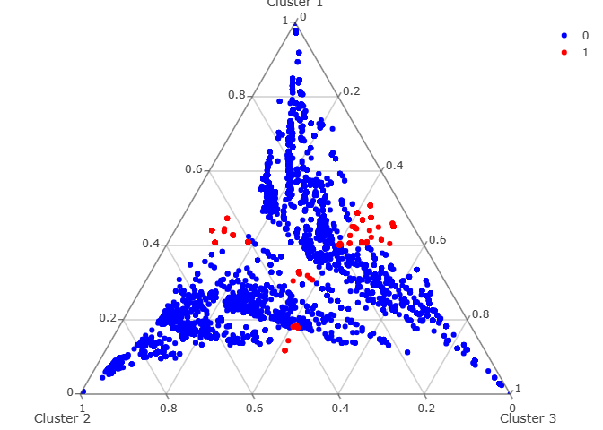
After performing the cluster analysis, we obtained three different and well-defined clusters. Since we used a fuzzy algorithm, it is necessary to define when an observation can be considered as fuzzy, meaning that it doesn’t belong to any cluster. In this case study, we followed the guidelines provided by Maharaj et al. [18] in 2022: “a case is considered to have fuzzy membership in two clusters if the membership degrees are less than 0.6 in one cluster and greater that 0.4 in the other cluster. A case is considered to have fuzzy membership in all three clusters if the membership degrees are less than 0.4 but greater than 0.3 in all three clusters.”

Following these guidelines, we found out that in our dataset 1,202 observations were fuzzy, representing the 18.7% of the total observations of the dataset. As mentioned above, we found three different clusters; we shared the results of this analysis with the company, to check the alignment between the outcomes of the analysis and what people in production observe on the production line every day, and the feedback was positive.

Figure 3 represents the ternary plot of the cluster analysis that was performed: the red dots represent the fuzzy observations, which were discarded.

4. 4. Predictive models

In relation to predictive models, we followed a two-step methodology.

To begin with, we evaluated the effectiveness of nine distinct ML models utilizing the complete dataset derived from the cluster analysis. Following this initial phase, we identified and select the top-performing model. Subsequently, we directed our efforts towards the approach outlined in Section 3, specifically the Fuzzy model, in which dedicated ML models were constructed for each cluster, employing the most proficient ML model identified in the previous phase. We implemented this approach and compared its results with the baseline approach.

The metric used to evaluate the performances of the model, referring to the first step, and the Fuzzy model approach, referring to the second step, was the Mean Absolute Percentage Error (MAPE). The equation to calculate this metric is presented in Eq. 1 as:

(1)

Where y_i is actual value, is the forecast value and n is the number of observations.

In the first phase, we used the R Caret package to conduct an analysis to determine which model, among the nine presented in Table 2, performed better in a classical training-testing approach.

The results of this analysis are presented in Table 3.

Table 2. List of ML models evaluated.

ML model name	Corresponding caret method name
Linear regression	lm
Random Forest	Ranger
eXtreme Gradient Boosting	xgbTree
Elasticnet	enet
Bagged CART	treebag
Boosted Tree	blackboost
SVM with Linear Kernel	svmLinear
SVM with Radial Basis Function Kernel	svmRadial
Multivariate Adaptive Regression Splines	earth

Table 3. Comparison of the different ML models in predicting the PLT

ML model	MAPE
Linear regression	0,11375402
Random Forest	0,07938010
eXtreme Gradient Boosting	0,08963411
Elasticnet	0,1129337
Bagged CART	0,11279711
Boosted Tree	0,11517795
SVM with linear kernel	0,09969439
SVM with Radial Basis Function Kernel	0,09624472
MARS	0,11352352

As it is possible to observe from Table 3, it emerged that the top-performing model was the Random Forest, as it has the minimum MAPE among the nine tested models.

This outcome aligns with the findings of Rizzuto et Al.[10], Lingitz et Al.[1] and Pfeiffer et Al.[6], confirming that this model is indeed very accurate when it comes to predict lead time.

So, to check the effectiveness of the methodology proposed in Section 3, the Fuzzy Model, we utilized Random Forest.

We compared the results obtain by adopting this methodology with the ones achieved by the baseline approach. Table 4 represents the results of our analysis. Also here, as mentioned earlier, the metric used for performance comparison was MAPE.

Table 4. Comparison of the Fuzzy model with the baseline approach

Approach	MAPE RF
No cluster	0,07938010
Fuzzy model	0,06769214

Analysing the results in Table 4, it is possible to observe that the Fuzzy model approach outperform the baseline approach, indeed, it obtains a lower MAPE.

5. Discussion

The results obtained from this study can be divided into two main branches: in the first, we focused on understanding which ML model, among the nine tested, was most suitable for achieving the best possible prediction of PLT.

The second branch concerns the application of fuzzy clustering as a sort of pre-processing step. This methodology was tested, following the guidelines provided in Section 3, to determine if this option could indeed provide predictive improvements, compared to the baseline approach.

To begin, we were able to confirm that the Random Forest emerged as the best ML model, as it accurately predicts the PLT. It is essential to emphasize that this result aligns with our findings in the brief literature review we conducted.

Indeed, from the analysis of three similar cases to ours, it was evident that Random Forest was the most precise ML model among those evaluated.

Regarding the use of clustering as a pre-processing step, we tested the approach described in section 3, Fuzzy model, in combination with Random Forest, comparing it with the baseline approach, to understand if there were some improvements.

By testing this approach, fuzzy model, which involves using weighted datasets derived from the initial dataset where the membership degree of each observation to each cluster is used as weight, we found that, it may provide some improvements in predictions.

Concerning Random Forest, we should underline that it is a very valid and accurate ML model, representing the state of the art in various field: this makes it challenging to improve this model. However, the fact that the Fuzzy model approach outperforms the sole application of Random Forest in the analysed case study encourages us to explore this methodology further in our future works.

6. Conclusions and future works

This study focuses on the presentation of an innovative predictive methodology that integrate the fuzzy C-medoids clustering algorithm and predictive models to enhance the predictive performance in the case of PLT.

We developed this work around a case study in collaboration with a company, working in the fashion industry. The main goal of this work was to obtain the most accurate prediction of PLT, for a productive process.

Initially, it was necessary to identify the best performing ML model on the data: this analysis showed that Random Forest remains a highly reliable and accurate model when the goal is to obtain accurate PLT forecasts.

We then applied the approach described in Section 3, which combines fuzzy clustering and predictive models, in order to test whether this approach offered any advantages in terms of predictive accuracy. This analysis showed that this approach can provide advantages in terms of predictive accuracy.

Clearly, since our analysis is based on a case study, we cannot generalise the results obtained. Instead, it is very useful as a starting point for a broader research direction.

ACKNOWLEDGMENTS

Authors would like to thank the leading multinational company in the fashion industry that funded this project and provided the data analysed in this project. In particular, the authors thank Barbieri Pietro, Bortolan Luca, Canale Matteo, Giada Marco, Longi Davide, Napol Fabio, Paganin Danny for their invaluable suggestions.

This study was carried out within the MICS (Made in Italy—Circular and Sustainable) Extended Partnership and received funding from the European Union Next-GenerationEU (PIANO NAZIONALE DI RIPRESA E RESILIENZA (PNRR)—MISSIONE 4 COMPONENTE 2, INVESTIMENTO 1.3—D.D. 1551.11-10-2022, PE00000004). This manuscript reflects only the authors’ views and opinions; neither the European Union nor the European Commission can be considered responsible for them.

This study was carried out within the MOST—Sustainable Mobility National Research Centre and received funding from the European Union Next-GenerationEU (PIANO NAZIONALE DI RIPRESA E RESILIENZA (PNRR)—MISSIONE 4 COMPONENTE 2, INVESTIMENTO 1.4—D.D. 1033 17 June 2022, CN00000023). This manuscript reflects only the authors’ views and opinions, neither the European Union nor the European Commission can be considered responsible for them.

References

[1] L. Lingitz et al., "Lead time prediction using machine learning algorithms: A case study by a semiconductor manufacturer," Procedia Cirp, vol. 72, pp. 1051-1056, 2018. View Article
[2] Y. Meidan, B. Lerner, G. Rabinowitz, and M. Hassoun, "Cycle-time key factor identification and prediction in semiconductor manufacturing using machine learning and data mining," IEEE transactions on semiconductor manufacturing, vol. 24, no. 2, pp. 237-248, 2011. View Article
[3] P. Backus, M. Janakiram, S. Mowzoon, C. Runger, and A. Bhargava, "Factory cycle-time prediction with a data-mining approach," IEEE Transactions on Semiconductor Manufacturing, vol. 19, no. 2, pp. 252-258, 2006. View Article
[4] J. Wang, J. Zhang, and X. Wang, "A data driven cycle time prediction with feature selection in a semiconductor wafer fabrication system," IEEE Transactions on Semiconductor Manufacturing, vol. 31, no. 1, pp. 173-182, 2018. View Article
[5] I. Tirkel, "Cycle time prediction in wafer fabrication line by applying data mining methods," in 2011 IEEE/SEMI Advanced Semiconductor Manufacturing Conference, IEEE, 2011, pp. 1-5. View Article
[6] A. Pfeiffer, D. Gyulai, B. Kádár, and L. Monostori, "Manufacturing lead time estimation with the combination of simulation and statistical learning methods," Procedia Cirp, vol. 41, pp. 75-80, 2016. View Article
[7] J. Wang and J. Zhang, "Big data analytics for forecasting cycle time in semiconductor wafer fabrication system," International Journal of Production Research, vol. 54, no. 23, pp. 7231-7244, 2016. View Article
[8] J. Bender and J. Ovtcharova, "Prototyping machine-learning-supported lead time prediction using AutoML," Procedia Computer Science, vol. 180, pp. 649-655, 2021. View Article
[9] A. Öztürk, S. Kayalıgil, and N. E. Özdemirel, "Manufacturing lead time estimation using data mining," European Journal of Operational Research, vol. 173, no. 2, pp. 683-700, 2006. View Article
[10] A. Rizzuto, D. Govi, F. Schipani, and A. Lazzeri, "Lead Time Estimation of a Drilling Factory with Machine and Deep Learning Algorithms: A Case Study.," in IN4PL, 2021, pp. 84-92. View Article
[11] B. Ari and H. A. Güvenir, "Clustered linear regression," Knowledge-Based Systems, vol. 15, no. 3, pp. 169-175, 2002. View Article
[12] S. Trivedi, Z. A. Pardos, and N. T. Heffernan, "The utility of clustering in prediction tasks," arXiv preprint arXiv:1509.06163, 2015.
[13] R. Krishnapuram, A. Joshi, O. Nasraoui, and L. Yi, "Low-complexity fuzzy relational clustering algorithms for web mining," IEEE transactions on Fuzzy Systems, vol. 9, no. 4, pp. 595-607, 2001. View Article
[14] N. K. Nagwani and S. V. Deo, "Estimating the concrete compressive strength using hard clustering and fuzzy clustering based regression techniques," The Scientific World Journal, vol. 2014, 2014. View Article
[15] M. Disegna, P. D'Urso, and F. Durante, "Copula-based fuzzy clustering of spatial time series," Spatial Statistics, vol. 21, pp. 209-225, 2017. View Article
[16] X. L. Xie and G. Beni, "A validity measure for fuzzy clustering," IEEE Transactions on Pattern Analysis & Machine Intelligence, vol. 13, no. 08, pp. 841-847, 1991. View Article
[17] J. C. Gower, "A general coefficient of similarity and some of its properties," Biometrics, pp. 857-871, 1971. View Article
[18] E. A. Maharaj, L. D. Giovanni, P. D'Urso, and M. Bhattacharya, "Deployment of Renewable Energy Sources: Empirical Evidence in Identifying Clusters with Dynamic Time Warping," Social Indicators Research, pp. 1-22, 2022. View Article