Journal of Machine Intelligence and Data Science (JMIDS)

1. Introduction

Companies want to understand their customers in the best possible way, in order to reduce customer churn (when a customer stops buying products from the company) for example. It is sometimes said that the goal is for the company to obtain a full 360 degrees view of the customers. Companies have some categorical data, such as Net Promoter Score from their customers from internal surveys, where they ask how likely a customer is to recommend the products of the company to other people. However, there is a lot of useful information in the text in social media posts, internal feedback forms, and posts on review sites about companies written by customers. To gain insight from the unstructured text, written by customers, techniques such as topic modelling are required. The extraction of topics from unstructured text can also be potentially used as features in classifiers. The practical importance of topic modelling and text clustering has increased in recent years, due to continuing expansion of internet usage world-wide, which lead to increasing amount of text data stored and collected online as well as in internal data bases of businesses.

The aim of statistical topic modelling is to extract and summarize trending issues from a corpus of text documents in the form of a set of “themes” or topics that occur in it [1]. Topic modelling methods include Latent Dirichlet Allocation (LDA) [2] and Gibbs Sampling Algorithm for a Dirichlet Mixture Model (GSDMM) [3]. It is also possible to use cluster techniques with word embedding of text to do topic modelling. LDA is one of the most popular topic modelling methods and it uses a generative assumption that a document is created from different proportions of multiple topics [4]. The Dirichlet Mixture Model has been designed for short text topic modelling and it provides one topic per document which effectively results in text clustering. While LDA works better for long text collections such as essays and articles, GSDMM is more suitable for shorter text [5, 4] such as tweets, comments on social media and customers’ reviews.

Generally, model evaluation involves measuring how homogeneous the topics are, by assessing whether each topic or cluster contains similar words or documents, so the more homogeneous content in any cluster the better the result. In practice, the evaluation process for GSDMM model, including the task of tuning its hyper-parameters, is challenging as the conventional evaluation methods do not have implementations that would be easy to apply and often do not result in intuitive topics.

The GSDMM algorithm has three hyper-parameters: α, β and K, where α is the parameter of the Dirichlet prior related to topics, β is the parameter of the Dirichlet prior related to words [6] and K is the upper bound on the number of topics. Following the work of [3] where the method was introduced, many researchers and practitioners use α=β=0.1 as the default setting for the GSDMM algorithm [7, 4, 8, 9, 5, 10]. Alternatively, the choice is based on manual empirical experiments by testing several combinations of values and picking the one that gives the most informative or useful topics [1].

As pointed out in [11], the choice of the values for α and β is important as it can have a big impact on the fitted model. For example, the magnitude of β influences the number of discovered topics, with bigger β leading to a smaller number of topics. Therefore, there is a real need to develop methods for tuning of these hyper-parameters, as the practice adopted by many authors to date is not optimal. Evaluating topic models is a difficult task given the unsupervised nature of such models as well as the complexity of text data.

This project is part of a larger research program to build machine learning models for customer churn in the telecommunication industry. The machine learning models to predict customer churn of telecom users, typically reported in the literature, involve structured data with numerical and categorical variables [26, 27, 28, 29, 30] or customer segmentation [31, 32]. Recently, [33] built a churn model that employed unstructured data and social network analysis.

This paper is focused on topic modelling evaluation methods in the context of unsupervised learning, to bridge a gap in the existing body of research and provide more tools for practitioners. New evaluation methods for the GSDMM algorithm are proposed and their performance compared with UMass coherence in empirical experiments. The proposed method involves converting the words that represent each discovered topic into numerical vectors using a word embedding. Next, the between-topic and within-topic distances are calculated. We present a case study using online comments generated by customers of British telecommunication industry.

In the presented case study, the topics obtained through the optimised GSDMM model are compared with those resulting from the K-means algorithm applied to the word embeddings of text. To the best of our knowledge, there are no published studies that rigorously examine the performance of text topic modelling methods, particularly the GSDMM algorithm, on text data generated by customers of British telecommunication industry.

2. Related Work

A conventional method of evaluating topic models is the perplexity of a held-out test set [2, 12], defined as the likelihood of the test set given the training set. It has been pointed out in literature that perplexity does not necessarily lead to understandable topics, showing poor correlation with human-labelled data [13, 14]. In the recent years, many methods focus on the semantic coherence of topics as the preferred evaluation metric. The two state-of-the-art ways of calculating topic coherence are the UCI topic coherence [15] using Point Mutual Information (PMI) [16] and UMass topic coherence [17]. The UCI topic coherence requires an external database. In the context of topic modelling for short text, the UCI topic coherence was used by [14, 18, 19, 10]. The UMass topic coherence was used in the context of topic modelling for short text by [20] and [4]. Recently, [21] proposed to evaluate topic models by simulating labelled pseudo-documents based on the probability distributions that are provided by the fitted topic model. However, as mentioned by several authors [18, 14, 22], evaluating topic modelling is still an open problem.

In the literature on short text topic modelling, popular types of text datasets frequently analysed by researchers include news data [9, 3, 8, 5] or web search snippets [19, 10, 23, 24, 25]. In recent years, analyses focused on the COVID-19 pandemic have been popular [7, 21, 1]. [4] used a corpus of news articles about markets and companies obtained from a financial magazine, a dataset of tweets about the weather, and tweets about the August GOP debate that took place in Ohio in 2015.

3. Methodology

In this section, the proposed methodology for analysing telecom customers' views is described. This involves the Dirichlet Mixture Model (DMM) that is used for topic discovery in short text documents. Moreover, the application of word embedding and metrics to evaluate the resulting clusters of documents are presented.

3. 1. Definitions and Notation

We begin with basic definitions and notation needed to describe a topic model.

A corpus is defined as a collection of documents and a document - a collection of words, also referred to as terms. The set of all words from the entire corpus is called the vocabulary. Below, we define the basic notation that is used in this section:

V – the number of words in the vocabulary,
wv – the v^th word in the vocabulary, v = 1, …, V,
D – the number of documents in the corpus,
d – a document label, d = 1, …, D,
Nd – the number of words in document d,
wd,i – the i^th word in document d, where i = 1, …, N_d,
K – the number of topics/clusters in the corpus,
k – a topic/cluster label, k = 1, …, K,
z_d – the topic assigned to document d, z_d = 1, …, K.

We assume that the aim is to assign exactly one topic to each document. Therefore, topics can be viewed as non-overlapping clusters of documents. Below, we fix the notation for the distributions of topics and words in a corpus.

Let θ₁, …, θ_K ≥ 0, where θ₁ + …+ θ_K = 1, be the probability distribution over topics for the whole corpus. In other words, for a randomly chosen document d, the probability of it being in the cluster k is given by θ_k. Let θ = (θ₁, …, θ_K) be the vector of topic probabilities.

Mathematically, a topic is defined as a probability distribution over words. Let φ_k,1, φ_k,2, …, φ_k,V ≥ 0, where φ_k,1 + φ_k,2 + …+ φ_k,V  = 1, be the probability distribution over words for topic k. Let φ_k = (φ_k,1, φ_k,2, …, φ_k,V) be the vector of word probabilities for topic k.

3. 2. Dirichlet Multinomial Mixture Model

Dirichlet Multinomial Mixture (DMM) model [34] assumes that the vectors of proportions θ and φk are realisations of random variables having a Dirichlet distribution, while topics and words come from Multinomial distributions.

Given priors α and β for the Dirichlet distributions, each document d is assumed to have been generated in the following steps.

Step 1: Sample a vector of topic proportions θ from the K-dimensional Dirichlet(α,…, α) distribution.

Step 2: For each topic k = 1, …, K, sample a vector of word proportions φk related to that topic from the V-dimensional Dirichlet(β,…,β) distribution.

Step 3: For each document d = 1, …, D:

1. Sample one topic z_d ~ Multinomial(θ).
2. For i = 1, …, N_d, sample a word w_d,i ~ Multinomial(φ_zd).

Therefore, once z_d is known, the document is generated as a sequence of words which are independent of one another and come from the same distribution. Parameter α is related to topics' distribution while parameter β is related to words' distribution. The DMM model assumes the same values of α for all topics and the same values of β for all words. [3] proposed a collapsed Gibbs Sampling Algorithm for the DMM model, denoted as GSDMM, that is an efficient implementation of the method in terms of its convergence. The authors noted that for a given K the algorithm may result in some of the clusters/topics being empty (i.e. with no documents assigned to them).

The subsequent 350 trading days, starting from April 28, 2021, for the NASDAQ 100 and the Dow Jones, and from May 7, 2021, for the DAX, up to September 15, 2022, were designated for testing. This represents roughly 11% of the entire dataset for all three indices.

3. 3. Proposed Model Evaluation Metrics

To determine the hyper-parameters of the various topic modelling algorithms, such as the number of topics, a cost function is required. For topic modelling, the within-cluster variation of words (WCV) should be minimized and the between-cluster variation (BCV) of words should be maximized. We consider a linear scalarization of them to create the cost function:

(1)

where 0 ≤ 𝜆 ≤ 1 is a fixed constant. This cost function is then minimised. In particular, for 𝜆=1 this cost function is related to the well-known measure used in the algorithm of K-means clustering [35].

3.3.1. Word Embedding

To find the values of WCV and BCV, the words in clusters are first represented as numerical vectors using a word embedding algorithm. Ideally, a word embedding is a type of numerical representation of words designed such that words with similar meaning have a similar representation [36]. Two popular tools to construct embedding values are the so-called Word2Vec method [37] and BERT model [38]. Auxiliary word embeddings were utilised by [19] and [10] in the Poisson DMM model to promote words that are semantically related during the model fitting process. Also, [9] used latent feature word representation to incorporate external information into LDA and DMM models for short text and/or small sample size. The authors used Google word vectors and Stanford vectors.

In this paper, we chose the embedding FastText created by Facebook's AI Research (FAIR) lab using a pre-trained word vectors [39]. Thus, each word wi in the corpus is represented as an m-dimensional vector ei, where m = 300 in our experiments.

3.3.2. Within-topic Variation

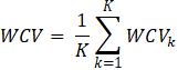
For a given topic/cluster k, the within-cluster variation can be measured by

(2)

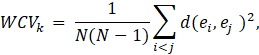
where d(e_i, e_j) is the distance between the two numerical vectors and N is a fixed number of most frequent words. Here, we set N = 10, similarly to the practice of [14] for PMI measure, and [15] who defined a topic by its top ten words. For the distance d(e_i, e_j), measures such the Euclidean distance (using L2 norm), the Manhattan distance (using L1 norm) or a correlation-based distance can be used. Then, the overall within-cluster variance is found as the average

(3)

3.3.3. Separation between Topics

The between-cluster variance is calculated by finding distances between clusters which can be done in several ways. We consider the following four measures to represent the distance between two clusters:

1. the average distance between all possible pairs of the top N words in each cluster,
2. the distance between centroids of the two clusters,
3. the minimal distance between all possible pairs of the top N words in each cluster (related to the well known single linkage),
4. the maximal distance between all possible pairs of the top N words in each cluster (related to the well known complete linkage).

These measures are known by their use in the hierarchical clustering algorithm [40].

Then, the overall between-cluster variance is found as the average

(4)

where BCV_k,j is the separation measure between clusters k and j, obtained by using one of the approaches (a) – (d).

4. Empirical Experiments

In this section, empirical experiments are performed on the datasets obtained from social media platforms and related to the views of the customers of British telecom industry. After cleaning the data, topic models are fitted using the GSDMM algorithm. Model evaluation metrics proposed in section 3.3 are implemented and analysed. Moreover, the obtained topics are compared with text clusters resulting from the K-means algorithm.

To explore views of British telecom customers using the proposed methodology, text data were scraped from two online platforms: TrustPilot (http://www.trustpilot.com/) and BT Community website (http://community.bt.com/). A dataset with 1,979 customers’ comments related to Vodafone was obtained from the TrustPilot website and 1,506 comments of BT’s individual customers were downloaded from the BT Community website.

4. 1. Data Pre-Processing

The two datasets have been pre-processed and cleaned using the following pipeline: (1) convert all letters to lower case; (2) remove all non-alphanumeric characters including punctuation; (3) remove all words that do not appear in the English Dictionary; (4) remove stop words; (5) remove digits; (6) remove one-letter words; (7) remove documents that contain only one word. For step (3), Python's FastText Word Embedding library was used. The words removed in this step were mostly misspelled words. We did not use automatic spelling correction due to the dangers and limitations of the existing methods as pointed out in [41].

4. 2. Data Exploration

Table 1 shows summaries of the datasets before and after cleaning, respectively. Before cleaning, the average number of words per document was between 98 and 115 words across the datasets, while after cleaning between 40 and 49 words. Around 43% of words were stop words. Histograms, shown in Figures 1 and 2 in the Appendix, revealed that the distributions of the number of words per document are right-skewed with the vast majority of text documents shorter than 50 words.

Table 2 presents the most frequent words and bi-grams, respectively, in the documents after cleaning. Unsurprisingly, the name of the company appears as one of the top words. For Vodafone, the word ‘phone’ and the bigram ‘customer service’ stand out indicating that issues related to either phones or contacting the customer service via phone are frequently mentioned. Moreover, the negation words such as ‘no’, ‘not’, ‘no one’, ‘still not’ are present which may indicate negative sentiments in customers’ comments. Also, words related to specific services such as ‘tv’ or ‘smart hub’ can be observed.

Table 1: Summaries of the telecom datasets before (BC) and after (AC) cleaning. The columns show: the number of text documents, the mean number of words per document before and after cleaning, respectively, minimum and maximum number of words per document after cleaning and the total percentage of stop words.

Dataset	Sample size	Mean BC	Mean AC	Min AC	Max AC	Stop words
BT Community	1,506	98	40	2	541	42.8%
Vodafone	1,979	115	49	2	397	44.4%

 

Table 2: The most frequent words and bigrams in the telecom datasets after cleaning.

BT Community dataset
Top words	bt, td, not, get, no, would, up, new, now, tv
Top bigrams	bt tv, smart hub, bt sport, digital voice, set up
Vodafone dataset
Top words	not, vodafone, phone, customer, no, service, get, contract, told, would
Top bigrams	customer service, no one, even though, customer services, still not

4. 3. Design of Experiments

We explore several cost functions to evaluate clustering of documents into topics. The list of the considered metrics and the notation used to refer to them in this section is given in Table 3. In our empirical experiments, Euclidean distance was used for d(ei, ej) in formula (2) to compute the cost functions.

Table 3: Model evaluation metrics used in empirical experiments based on formula (1).

Notation	𝜆	Description
WCV	1	using formula (3)
MeanBCV	0	using the distance between centroids of the two clusters
MinBCV	0	using the minimal distance between all possible pairs of the top N words in each cluster
MaxBCV	0	using the maximal distance between all possible pairs of the top N words in each cluster
CohBCV	0	using UMass Coherence
MeanCF	0.5	using the distance between centroids of the two clusters
MinCF	0.5	using the minimal distance between all possible pairs of the top N words in each cluster
MaxCF	0.5	using the maximal distance between all possible pairs of the top N words in each cluster
CohCF	0.5	using UMass Coherence

The GSDMM algorithm for topic discovery is applied to the two text corpora. Each model evaluation criterion is optimised with respect to the hyper-parameters α and β using a grid of the values between 0.05 and 1 with step 0.05, while the parameter K stays fixed and equal to K = 5.

Moreover, for each resulting clustering into topics, we calculate the quantity

(5)

where K is the number of topics/clusters and n_i is the number of documents in the i^th cluster. This measures how balanced the resulting clusters are in terms of their relative sizes, with size_b = 0 when each topic has the exact same number of documents in it.

Part of the workflow of our proposed evaluation method of the GSDMM is to convert the text into vectors using word embedding. Clustering methods such as K-means or DBSCAN can be used on numerical vectors to determine clusters that define the topics. We investigate the use of K-Means clustering algorithm with the embedded vectors and compare the results to those from the optimized GSDMM. The K-means clustering algorithm is applied on the embedded text data, using the same text embedding from the FastText library as for the GSDMM evaluation measure, with the number of clusters set to 5 for easy comparison.

4. 4. Results

4. 4. 1 Analysis of the optimal hyper-parameters

Table 4 shows the optimal values of α and β for each one of the considered criteria. We observe that generally most cost functions yield similar optimal hyper-parameters, with the exception of the cost function MaxCF and MaxBCF. Moreover, it can be seen that majority of the optimal values for both hyper-parameters are greater than 0.5, and often α_opt is smaller than the corresponding β_opt. The meaning of parameter α is that it controls how easily a cluster gets removed when it becomes empty, that is if α=0 then a cluster will never be re-populated once it gets empty. On the other hand, β controls how easily words join clusters and if β=0 then a word will never join a cluster without extremely similar words in it. Our results suggest that the optimal models tend to create a moderately small number of clusters and the words can join them relatively easily during the estimation process.

Moreover, we noticed that when the number of clusters K was increased to 10, 15 and 20, it lead to many empty clusters, which in result yielded the same clustering with just 5 non-empty clusters.

Table 4: The optimal values of hyper-parameters α and β for various cost functions, where K=5 for GSDMM algorithm.

	BT Community dataset	αopt	βopt	Vodafone dataset	αopt	βopt
WCV		0.85	0.9		0.8	0.91
MeanBCV		0.6	0.75		0.35	1.0
MinBCV		0.9	0.95		0.5	0.65
MaxBCV		0.85	0.9		0.3	0.05
CohBCV		0.85	0.85		0.75	0.35
MeanCF		0.85	0.9		0.8	0.9
MinCF		0.75	0.95		0.8	0.9
MaxCF		0.05	0.9		0.4	0.5
CohCF		0.85	0.9		0.8	0.9

Table 5 shows the summaries of size_b that measures the balance of the clusters with respect to their sizes, that is the number of documents in each cluster. Based on the table, we conclude that when the hyper-parameters α and β vary, the resulting cluster sizes also vary, which indicates that different values of the hyper-parameters lead to considerably different clusters. This again suggests that using fixed values of the hyper-parameters, which is a commonplace in the literature, may not be the best practice.

Table 5: The summary statistics for size_b, defined in equation (5), for obtained clusters over the grid of α and β values for GSDMM.

Minimum	Maximum	Mean	Std deviation
BT Community data
0.04	1.2	0.47	0.26
Vodafone data
0.43	1.6	1.36	0.29

4. 4. 2 Analysis of the discovered topics

Tables 6 and 7 show the topics discovered in the datasets when K = 5 and with the optimal values of α and β according to the MeanCF criterion, as well as the topics discovered by the K-means algorithm.

For the optimised GSDMM, we observe that the clustering is balanced as the numbers of documents in each topic are very similar, with the exception of one very small cluster for Vodafone dataset. For the BT dataset, the five topics discovered using optimised GSDMM are related to:

1. connecting internet devices (‘connect’, ‘hub’, ‘router’, ‘wifi’),
2. tv services (‘tv’, ‘sport’, ‘watch’),
3. communication (‘email’, ’message’, ’send’),
4. phone service (‘number’, ‘phone’, ‘order’),
5. internet speed (‘speed’, ‘line’, ‘fibre’),

and the topics seem to be distinctive and well defined. For comparison, Table 8 in the Appendix shows the top words for five discovered topics for the same dataset when the fixed values α = β = 0.1 are used. Looking at the last column of the table, it can be observed that there are four clusters roughly similar in size and one very small cluster. The smallest cluster, labelled as Topic 4 in the Table 8, is related to tv services (‘tv’, ‘sport’, ‘watch’), and it contains only 4.3% of documents assigned to it, while for the optimised GSDMM the corresponding cluster contained 20.5% of documents (Topic 2 in Table 6 and Topic 4 in Table 8). Some other topics also can be matched between the optimised GSDMM results and Table 8, for example connecting internet devices (Topic 1 in Table 6 and Topic 3 in Table 8). However, some of the clusters created by the GSDMM with fixed values α = β = 0.1 seem to overlap with one another and be less focused, for example Topic 1 in Table 8 seems to be a mixture of broadband speed and phone lines and it overlaps with Topic 5 in Table 8. In conclusion, for these data, our optimised GSDMM model provided more focused and distinctive topics in comparison to the topics resulting from the GSDMM with fixed values α = β = 0.1.

Table 6: Top words for topics obtained by GSDMM for K=5 and α=α_opt, β=β_opt and by K-means for the BT Community dataset. The last column shows the proportion of documents in each topic.

Model	Top Words	Cluster size
Topic 1
GSDMM	connect, hub, work, phone, router, try, wifi, disc, use, device	21.4%
K-means	td, bt, not, hub, get, no, would, up, new, phone	44.4%
Topic 2
GSDMM	tv, sport, watch, channel, app, box, try, package, use, sky	20.5%
K-means	bt, tv, box, not, sport, now, watch, app, pro, get	19.7%
Topic 3
GSDMM	email, try, message, account, send, address, use, receive, access, help	19.7%
K-means	bt, email, not, get, no, account, new, number, phone, message	30.3%
Topic 4
GSDMM	number, phone, order, tell, service, broadband, thank, receive, try, email	19.8%
K-means	board, topics	1.0%
Topic 5
GSDMM	speed, line, fibre, engineer, connection, broadband, connect, hub, issue, work	18.6%
K-means	norton, bt, get, mcafee, not, spam, trying, server, tried, protect	4.5%

For the Vodafone dataset, the four main topics discovered by the optimised GSDMM are related to:

1. contacting customer service (‘phone’, ‘customer’, ‘tell’),
2. contracts (‘contract’, ‘month’, ‘pay’),
3. phones (‘phone’, ‘order’, ‘service’) and
4. company custom (‘company’, ‘custom’, ‘easily’),

with the last topic not being very focused and at the same time the largest. For these data, the clusters of documents are less distinctive. For comparison, Table 9 in the Appendix shows the top words for five discovered topics for the same dataset when the fixed values α = β = 0.1 are used. Again, in terms of the size of each cluster, a considerably different clustering is obtained when the fixed values of the hyperparameters are used for these data. Moreover, the topics are less distinctive and less focused when compared to the optimised GSDMM.

Table 7: Top words for topics obtained by GSDMM for K=5 and α=α_opt, β=β_opt and by K-means for the Vodafone dataset. The last column shows the proportion of documents in each topic.

Model	Top Words	Cluster size
Topic 1
GSDMM	customer, service, phone, vodafone, try, hour, contract, time, speak, chat	0.5%
K-means	broadband, not, service, no, internet, customer, get, worst, network, speed	6.7%
Topic 2
GSDMM	vodafone, phone, customer, tell, service, day, time, contract, hour, try	19.4%
K-means	vodafone, not, phone, customer, service, no, get, contract, after, now	28.3%
Topic 3
GSDMM	phone, vodafone, tell, customer, contract, order, cancel, service, send, day	18.8%
K-means	customer, phone, not, service, no, get, contract, chat, up, after	17.2%
Topic 4
GSDMM	vodafone, contract, customer, service, phone, pay, month, year, company, time	22.6%
K-means	not, vodafone, phone, no, customer, get, service, would, told, contract	43.9%
Topic 5
GSDMM	company, custom, easily, cow, submission, fund, contract, renew, crank, speech	38.7%
K-means	customer, service, worst, company, ever, not, bad, still, never, contract	3.8%

4. 4. 3 Comparison with K-means clustering

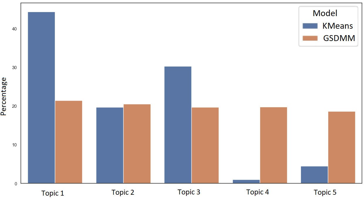
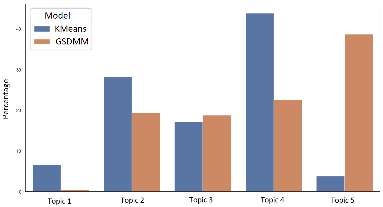
The clusters obtained from the optimized GSDMM and K-Means are not identical due to differences in algorithms, but we tried to match the five clusters from the two algorithms, as showed in Tables 6 and 7, depending on the most common words that exist in them. The relative sizes of the clusters within corpora, defined through the number of text documents for each discovered topic, are visualized in Figures 3 and 4 in the Appendix.

For the BT Community dataset, the first three topics showed in Table 6 match quite well between K-Means and GSDMM, as they contain similar keywords, and similar numbers of documents in them. Topics 4 and 5 do not seem to be similar. For the Vodafone dataset, the first four topics showed in Table 7 are quite similar between GSDMM and K-means, while the last topic does not seem to match.

Comparing the optimised GSDMM and K-Means, we can see that GSDMM produces clusters that are slightly more balanced in size than the K-Means algorithm. However, both methods produce some very small clusters in some cases. On the other hand, the optimised GSDMM seems to produce more homogeneous set of words within each topic, compared to K-Means which in most cases is not able to create a better clustering. For example, for BT Community dataset, we can find words such as ‘bt’, ‘not’ and ‘get’ in four out of five clusters obtained through K-Means, and cluster number 4 contains only 2 words.

7. Conclusion

We have investigated a method to evaluate the GSDMM model and to tune the two hyper-parameters α and β of the model. The method employs word embedding that uses externally pre-trained models for representing each word as a numerical vector in such way that words with similar meaning have similar numerical representations. Then, classical metrics for within-cluster variability and for separation between clusters can be applied. Using our model evaluation method, we find that the conventional values of the hyper-parameters α and β frequently used in the literature may not be optimal. In particular, for the text corpora related to telecom industry customers’ comments and opinions, the preferred values of the hyper-parameters tend to be between 0.5 and 1. Moreover, for these data, the discovered number of topics tends to be below 10. The proposed method and its implementation provide a solution for the challenging task of model evaluation and hyper-parameter tuning, without which the practical usefulness of the GSDMM method is limited.

We compared the topics obtained from GSDMM and the K-means clustering algorithm. Fairly similar topics were obtained from the two methods. However, the optimised GSDMM seems to produce more homogeneous set of words within each topic, in comparison to K-Means.

It should be noted that the obtained results and conclusions have a level of uncertainty related to them as they are based on a specific corpus and as such are due to random variations. Another source of uncertainty is related to the settings of the employed algorithms. In a recent paper [42], a visual method of presenting uncertainty for word clouds resulting from LDA model is proposed. Moreover, in the context of humanities research, the accuracy issues arising from assigning topic labels and topic interpretation are discussed in [43]. However, quantification of such uncertainties is currently an open area of future research.

In future work, we will investigate other word embedding techniques than FastText. Also, we plan to experiment with different clustering algorithms. Our general goal is to use the methods developed in this paper to include text data in classifiers for customer churn. Also, it may be interesting to investigate the use of large language models for topic modelling [44].

Acknowledgements

We thank David Yearling, Sri Harish Kalidass and Michael Free for discussions, particularly on sources of data sets.

References

5. Appendix

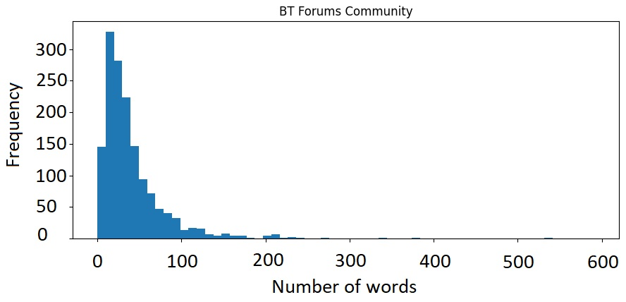
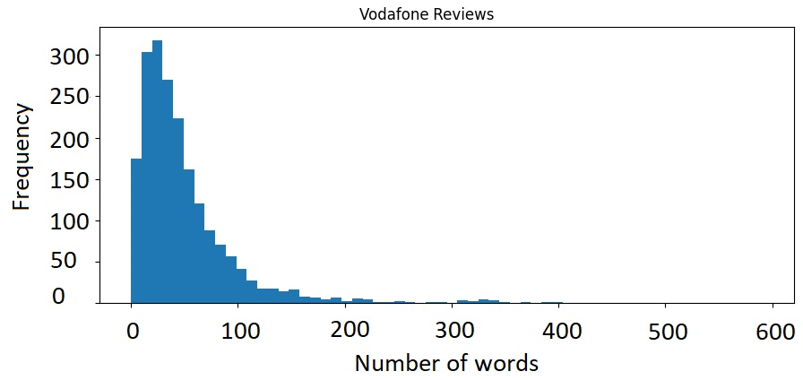
Table 8: Top words for the five topics for GSDMM with K = 5 and α = β = 0.1 for BT Community dataset. The last column shows the proportion of documents in each topic.

	Top Words	Cluster size
Topic 1	phone, speed, number, line, broadband, tell, work, order, service, fibre	20.5%
Topic 2	email, try, message, account, send, receive, address, thank, help, use	26.7%
Topic 3	hub, connect, try, work, router, wifi, phone, use, problem, disc	19.1%
Topic 4	tv, sport, watch, app, channel, try, box, package, sky, use	4.3%
Topic 5	cable, phone, speed, connect, wire, router, line, house, thank, socket	29.4%

 

Table 9: Top words for the five topics for GSDMM with K = 5 and α = β = 0.1 for Vodafone dataset. The last column shows the proportion of documents in each topic.

	Top Words	Cluster size
Topic 1	phone, vodafone, customer, tell, service, contract, day, time, try, hour	3.5%
Topic 2	service, vodafone, customer, contract, month, phone, pay, year, time, company	20.4%
Topic 3	customer, phone, service, vodafone, try, tell, hour, contract, time, speak	16.8%
Topic 4	pay, contract, vodafone, phone, month, year, charge, cancel, company, customer	4.6%
Topic 5	internet, vodafone, service, customer, time, broadband, tell, speed, issue, engineer	54.6%

References

[1] K. Garcia and L. Berton, “Topic detection and sentiment analysis in Twitter content related to COVID-19 from Brazil and the USA” Applied Soft Computing, vol. 101, pp. 107057, 2021. View Article
[2] D. M. Blei, A. Y. Ng, and M. I. Jordan, “Latent Dirichlet Allocation” J. of Machine Learning Research, vol. 3, pp. 993-1022, 2003.
[3] J. Yin and J. Wang, “A Dirichlet multinomial mixture model-based approach for short text clustering,” in Proceedings of the 20th ACM SIGKDD International Conference on Knowledge Discovery and Data Mining, 2014. View Article
[4] J. Mazarura and A. de Waal, “A comparison of the performance of latent Dirichlet allocation and the Dirichlet multinomial mixture model on short text,” in 2016 Pattern Recognition Association of South Africa and Robotics and Mechatronics International Conference (PRASA-RobMech), pp. 1-6, 2016. View Article
[5] Y. Zuo, C. Li, H. Lin, and J. Wu, “Topic modeling of short texts: a pseudo-document view with word embedding enhancement,” IEEE Transactions on Knowledge and Data Engineering, 2021. View Article
[6] S. Liang, E. Yilmaz, and E. Kanoulas, “Dynamic clustering of streaming short documents,” in Proceedings of the 22nd ACM SIGKDD International Conference on Knowledge Discovery and Data Mining, pp. 995-1004, 2016. View Article
[7] M. R. Khairiyah and C. A. Hargreaves, “Leveraging Twitter data to understand public sentiment for the COVID-19 outbreak in Singapore,” International J. of Information Management Data Insights, vol. 1, no. 2, pp. 100021, 2021. View Article
[8] R. Guan, H. Zhang, Y. Liang, F. Giunchiglia, L. Huang, and X. Feng, “Deep feature-based text clustering and its explanation,” IEEE Transactions on Knowledge and Data Engineering, 2022. View Article
[9] D. Q. Nguyen, R. Billingsley, L. Du, and M. Johnson, “Improving topic models with latent feature word representations,” Transactions of the Association for Computational Linguistics, vol. 3, pp. 299-313, 2015. View Article
[10] C. Li, Y. Duan, H. Wang, Z. Zhang, A. Sun, and Z. Ma, “Enhancing topic modeling for short texts with auxiliary word embeddings,” ACM Transactions on Information Systems (TOIS), vol. 36, no. 2, pp. 1-30, 2017. View Article
[11] T. L. Griffiths and M. Steyvers, “Finding scientific topics,” in Proceedings of the National Academy of Sciences of the United States of America, vol. 101 (Suppl 1), pp. 5228-5235, 2004. View Article
[12] H. M. Wallach, I. Murray, R. Salakhutdinov, and D. Mimno, “Evaluation methods for topic models,” in Proceedings of the 26th International Conference on Machine Learning, p. 139, 2009. View Article
[13] J. Chang, S. Gerrish, C. Wang, J. Boyd-Graber, and D. M. Blei, “Reading tea leaves: how humans interpret topic models,” in Proc. Int. Conf. Neural Inf. Process. Syst., pp. 288-296, 2009.
[14] Y. Zuo, J. Wu, H. Zhang, H. Lin, F. Wang, K. Xu, and H. Xiong, “Topic modeling of short texts: a pseudo-document view,” in Proceedings of the 22nd ACM SIGKDD International Conference on Knowledge Discovery and Data Mining, pp. 2105-2114, 2016. View Article
[15] D. Newman, J. Han Lau, K. Grieser, and T. Baldwin, “Automatic evaluation of topic coherence,” in Human Language Technologies: The 2010 Annual Conference of the North American Chapter of the ACL, pp. 100-108, 2010.
[16] K. Church and P. Hanks, “Word association norms, mutual information, and lexicography,” Computational Linguistics, vol. 6(1), pp. 22-29, 1990.
[17] D. Mimno, H. M. Wallach, E. Talley, M. Leenders, and A. McCallum, “Optimizing semantic coherence in topic models,” in Proceedings of the 2011 Conference on Empirical Methods in Natural Language Processing, pp. 262-272, 2011.
[18] J. Qiang, Z. Qian, Y. Li, Y. Yuan, and X. Wu, “Short text topic modeling techniques, applications, and performance: a survey,” IEEE Transaction on Knowledge and Data Engineering, vol. 34, pp. 1427-1445, 2022. View Article
[19] C. Li, H. Wang, Z. Zhang, A. Sun, and Z. Ma, “Topic modeling for short texts with auxiliary word embeddings,” in Proceedings of the 39th International ACM SIGIR Conference on Research and Development in Information Retrieval, SIGIR '16, (New York, NY, USA), pp. 165-174, Association for Computing Machinery, 2016. View Article
[20] J. R. Mazarura, Topic modelling for short text. MSc thesis, University of Pretoria, 2015.
[21] C. Weisser, C. Gerloff, A. Thielmann, A. Python, A. Reuter, T. Kneib, and B. Säfken, “Pseudodocument simulation for comparing LDA, GSDMM and GPM topic models on short and sparse text using Twitter data,” Comp. Stat., pp. 1-28, 2022. View Article
[22] D. M. Blei, “Probabilistic topic models,” Communications of the ACM, vol. 55, pp. 77-84, 2012. View Article
[23] M. Chen, X. Jin, and D. Shen, “Short text classification improved by learning multi-granularity topics,” in IJCAI, 2011.
[24] X.-H. Phan, L.-M. Nguyen, and S. Horiguchi, “Learning to classify short and sparse text & web with hidden topics from large-scale data collections,” in Proceedings of the 17th International Conference on World Wide Web, pp. 91-100, 2008. View Article
[25] A. Sun, “Short text classification using very few words,” in Proceedings of the 35th International ACM SIGIR Conference on Research and Development in Information Retrieval, SIGIR '12, pp. 1145-1146, 2012. View Article
[26] A. Idris, A. Khan, and Y. S. Lee, “Genetic programming and adaboosting based churn prediction for telecom,” in 2012 IEEE International Conference on Systems, Man, and Cybernetics (SMC), pp. 1328-1332, IEEE, 2012. View Article
[27] U. Ahmed, A. Khan, S. H. Khan, A. Basit, I. U. Haq, and Y. S. Lee, “Transfer learning and meta classification based deep churn prediction system for telecom industry,” arXiv preprint arXiv:1901.06091, 2019.
[28] U. Yabas, H. C. Cankaya, and T. Ince, “Customer churn prediction for telecom services,” in 2012 IEEE 36th Annual Computer Software and Applications Conference, pp. 358-359, IEEE, 2012. View Article
[29] J. Pamina, J. Beschi Raja, S. Sathya Bama, S. Soundarya, M. S. Sruthi, S. Kiruthika, V. J. Aiswaryadevi, G. Priyanka, “An effective classifier for predicting churn in telecommunication,” J. of Adv. Research in Dynamical & Control Systems, vol. 11, 2019.
[30] V. Umayaparvathi and K. Iyakutti, “Attribute selection and customer churn prediction in telecom industry,” in 2016 International Conference on Data Mining and Advanced Computing (sapience), pp. 84-90, IEEE, 2016. View Article
[31] M. Alkhayrat, M. Aljnidi, and K. Aljoumaa, “A comparative dimensionality reduction study in telecom customer segmentation using deep learning and PCA,” J. of Big Data, vol. 7, no. 1, pp. 1-23, 2020. View Article
[32] C. P. Chen, J.-Y. Weng, C.-S. Yang, and F.-M. Tseng, “Employing a data mining approach for identification of mobile opinion leaders and their content usage patterns in large telecommunications datasets,” Technological Forecasting and Social Change, vol. 130, pp. 88-98, 2018. View Article
[33] A. K. Ahmad, A. Jafar, and K. Aljoumaa, “Customer churn prediction in telecom using machine learning in big data platform,” J. of Big Data, vol. 6, no. 1, pp. 1-24, 2019. View Article
[34] K. Nigam, A. McCallum, S. Thrun, and T. M. Mitchell, “Text classification from labelled and unlabelled documents using EM,” Machine Learning, vol. 39, pp. 103-134, 2000. View Article
[35] D. J. C. MacKay, Information Theory, Inference and Learning Algorithms. Cambridge University Press, 2003.
[36] D. Jurafsky, J. H. Martin. Speech and Language Processing: An Introduction to Natural Language Processing, Computational Linguistics and Speech Recognition (2ed.), Prentice Hall, 2009.
[37] D. Karani, (2018) “Introduction to word embedding and word2vec,” [Online]. Available: View Article
[38] Q. Wang, P. Liu, Z. Zhu, H. Yin, Q. Zhang, and L. Zhang, “A text abstraction summary model based on BERT word embedding and reinforcement learning,” Applied Sciences, vol. 9, no. 21, pp. 4701, 2019. View Article
[39] B. Athiwaratkun, A. G. Wilson, and A. Anandkumar, “Probabilistic fasttext for multi-sense word embeddings,” arXiv preprint arXiv:1806.02901, 2018. View Article
[40] M. Halkidi, Y. Batistakis, and M. Vazirgiannis, “On clustering validation techniques,” J. of Intelligent Information Systems, vol. 17, pp. 107-145, 2001. View Article
[41] T. Kwartler, Text Mining in Practice with R. Wiley, 2017. View Article
[42] P. Winker, “Visualizing Topic Uncertainty in Topic Modelling”. arXiv preprint arXiv:2302.06482, 2023.
[43] M. Gillings, A. Hardie, “The interpretation of topic models for scholarly analysis: An evaluation and critique of current practice”. Digital Scholarship in the Humanities, vol. 38, no. 2, pp. 530–543, 2022. View Article
[44] D. Stammbach, V. Zouhar, A. Hoyle, M. Sachan, and E. Ash, “Re-visiting Automated Topic Model Evaluation with Large Language Models”. arXiv preprint arXiv:2305.12152, 2023.