Journal of Machine Intelligence and Data Science (JMIDS)

Volume 4 - Year 2023 - Pages 06-14
DOI: 10.11159/jmids.2023.002
Hybrid Models for Predicting Stock Market Performance
Iren Valova1, Natacha Gueorguieva2 Thakkar Aayushi 2, Pulluri Nikitha 2, Hassan Mohamed 2
1Computer and Information Science Department, University of Massachusetts Dartmouth
285 Old Westport Rd, Dartmouth, MA, USA, Iren.Valova@umassd.edu
2Department of Computer Science, College of Staten Island/City University of New York
2800 Victory Blvd, NY, USA, Natacha.Gueorguieva@csi.cuny.edu; Thakkar.Aayushi @cix.csi.cuny.edu;
Pulluri.Nikitha@cix.csi.cuny.edu; Hassan.Mohamed@cix.csi.cuny.edu
Abstract - Research on deep learning time series regression for stock market predictions and forecasting has grown exponentially in recent years. Considering the complexity of financial time series, combining deep learning with financial market prediction is regarded as a very important topic of research. The experiments in this study are divided into three settings which offer different topologies. For our first experimental setting we create hybrid sequential nonlinear models. For our second experimental setting we propose a new deep learning topology based on Attention CNN_BiLSTM for pretraining and light gradient boosting machine (LGBM) as a regressor (Attn_CNN_BiLSTM_LGBM). With our third experimental setting we propose a new model based on weighted average ensemble and the following four topologies: Attn_CNN_BiLSTM_LGBM, and attention_ CNN_ BiLSTM with various regressors. The ensemble model (EM) allows the contribution of each ensemble member to the prediction to be weighted proportionally to the performance of the EM. The latter achieves significantly better performance in predicting stock market.
Keywords: stock market prediction, convolutional neural networks, long-short term memory, gated recurrent unit
© Copyright 2023 Authors - This is an Open Access article published under the Creative Commons Attribution License terms. Unrestricted use, distribution, and reproduction in any medium are permitted, provided the original work is properly cited.
Date Received:2023-08-17
Date Revised: 2023-09-21
Date Accepted: 2023-09-26
Date Published: 2023-10-10
1. Introduction
Accurate stock market prediction is a challenging task due to the volatile and nonlinear nature of it which depends on numerous factors as local and global economic conditions, company specific performance and others. It is not possible to account all existing relevant factors which influence the stock market to make respective trading decisions without having appropriate algorithms and techniques.
Medium and large-sized companies play a significant role in the worldwide economy. Such companies make public offerings and gain a place on the stock exchange. Stocks, which dynamically update their price according to the company's current situation, also determine the company's value. The effect of human psychology on the movements of stocks cannot be underestimated. Technical stock interpretations have revealed that specific indicators affect the stock with various experiences from past to present.
Stock price prediction is one of four market categories defined in [1] which utilizes time-series data in order to calculate the anticipating values for stocks by researchers. Accurate stock market forecasting is considered as one of the most challenging problems among time series predictions due to the noise and high volatility associated with the data [2].
With the advancement of technology and science, there have been developments in artificial intelligence studies that have achieved success beyond human reasoning. Linear or nonlinear relations using tabular data, in particular, have become possible to be learned and applied by machine learning algorithms. In this context, the concept of machine learning can be considered a problem-solving method. Improved unique models, trained with the available datasets, can be implemented to real problems with high performance after their generalization and this applies also to solving stock price prediction.
Traditional machine learning methods such as artificial neural networks (ANNs) [3], tree-based models [4, 5] and support vector machines (SVM) [6] provide the necessary flexibly in modelling the existing nonlinear relationships. However, the performance of traditional machine learning methods largely depends on the selection of features, which affects the prediction capabilities of the model to a certain extent. In addition, there are some problems in applying these methods, such as poor generalization ability and slow convergence speed.
More recent studies of stock market forecasting problem are based on the current advances in deep learning (DL) models and techniques. DL has the important ability to better represent the complex nonlinear topologies and extract robust features what results in capturing the necessary relevant information from complex data. The latter allows stock market prediction using DL approaches to achieve better performance when compared to traditional machine learning methods. As deep learning models have improved, the methods used for predicting the stock market have shifted from traditional techniques to advanced deep learning techniques such as convolutional neural networks, recurrent neural networks, long short-term memory, gated recurrent units and graph neural networks (GNNs). CNNs capture important features using convolutional layers, making them effective at predicting stock fluctuations while the pooling layer effectively extracts the representative event history features [7].
Another popular neural network architecture – recurrent neural network (RNN) - is able to handle sequences of any length and capture long-term dependencies. The proposed LSTM and GRU architectures avoid the problem of gradient exploding or vanishing of the standard RNN learning better the long-term dependences. To conclude, CNN is able to learn local response from temporal or spatial data but lacks the ability of learning sequential correlations; on the other hand, RNNs are specialized for sequential modelling but are unable to extract features in a parallel way. The integration of CNN and LSTM further improves time series prediction and in particular the stock market forecast [8].
Most of the prediction models belong to a supervised learning approach, when training set is used for the training and test set is used for evaluation. Models based on semi-supervised learning as well as on different deep learning topologies as transfer learning, generative adversarial network (GAN) and reinforcement learning (RL) are still in development for being applied for stock market prediction [8]. The main tools used for implementation of DL models are Keras, TensorFlow, PyTorch, Theano, and scikit-learn [1].
Some researchers consider RL models as perspective and adaptable for stock market prediction because of the following two reasons: a) they do not need labelling of training data set; b) they use a reward function to maximize the return or minimize the risk. The latter however requires mathematical formulation of optimization objective criteria which needs to be conveyed in accordance with the specific task.
In this research we are using stock market dataset of China described in Section 4 of this paper. The experiments select the highest price, lowest price, opening price, closing price, trading volume, and adjusted closing price as features. In the training process, the number of different parameters such as number of layers and neurons, batch size, optimization, and activation functions, early stopping criteria etc. are properly refined to improve the model performance.
In Section 2 of this paper, we propose several new topologies which integrate CNN, stacked LSTM, GRU, BiLSTM and Attention CNN_BiLSTM with different regressor types. The last architectures are combined into weighted average ensemble model. In Section 3 we present the performance metrics used in our experiments. Experiments and results are discussed in Section 4. Section 5 concludes the study and outlines the future work.
2. CNN Models for Stock Market Prediction
Convolutional neural networks are most commonly used for classification of two-dimensional colour images. They belong to a class of neural networks which consist of an arbitrary number of convolutional and pooling layers, followed by one or more fully connected layers that perform classification. The purpose of pooling layers is to further reduce the output volume of each layer by performing a simple operation such as average, max and min.
The convolution improves machine learning algorithms in general because of its integrated capabilities: sparse interactions, sharing, and equivalent representations (translation invariance in image recognition framework). Sparse interaction is accomplished by using kernels (much smaller than the input) which occupy only a small fraction of pixels. Sharing of learned features by all neurons in a layer in the form of strides through the entire image leads to parameter sharing. The achievement of translation invariance originates from the identification of the learned features which is independent from their location [9].
The traditional convolutional layers use three-dimensional filters (kernels) and activation functions to process image features. However, in the stock prediction domain, CNNs are used to process time series data, which possess one dimensional features. To accommodate for this difference in data shape, CNNs for time series utilize a one-dimensional filter that slides over the time series with a stride determined by the dataset.
2.1. Gated Sequence Modelling with LSTM and GRU
CNNs however are unable to learn sequential correlations as they do not relay on historical data what is the case of time sequence-based models. In contrast, recurrent neural networks are specialized for sequential modelling but are unable to extract individual features in the same way as CNNs. RNNs are a family of neural networks for processing a sequence of values ![]() and some of them can also process sequences of variable length [10]. Recurrent computations in RNN which involve mapping inputs and parameters are formalized with computational graphs because of their repetitive configuration which corresponds to a chain of neural network (NN) events. Unfolding these graphs results in sharing of parameters across the RNN structure. Traditional RNNs suffer from both vanishing and exploding gradients and may fail when longer contexts are required in order to fit the model. As a result, a form of RNN, the GRU and long short-term memory were created for more efficient memory usage [11].
and some of them can also process sequences of variable length [10]. Recurrent computations in RNN which involve mapping inputs and parameters are formalized with computational graphs because of their repetitive configuration which corresponds to a chain of neural network (NN) events. Unfolding these graphs results in sharing of parameters across the RNN structure. Traditional RNNs suffer from both vanishing and exploding gradients and may fail when longer contexts are required in order to fit the model. As a result, a form of RNN, the GRU and long short-term memory were created for more efficient memory usage [11].
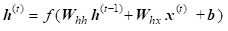
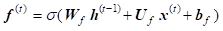
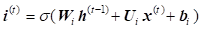
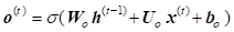
While standard RNN computes hidden layer at next time step directly using the input vector x , hidden state h, weight matrices w and vector b as shown below:
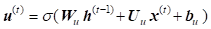
GRU first computes an update gate (another layer) which controls what parts of hidden state are updated vs. preserved:
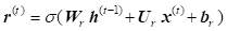
The next computations are on reset gate which determines what parts of the previous hidden state will be used to compute the new content:
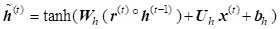
New hidden state content resets the gate selected useful parts of previous content:
Update simultaneously controls what is kept from previous hidden state and what is updated to the new hidden state:
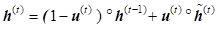
where ![]() and
and ![]() are the input and output vectors,
are the input and output vectors, ![]() - candidate activation vector,
- candidate activation vector, ![]() and
and ![]() are the
update and reset vectors;
are the
update and reset vectors; ![]() ,
, ![]() and
and ![]() are
weight matrices and bias vector parameters which need to be learned during
training;
are
weight matrices and bias vector parameters which need to be learned during
training; ![]() is sigmoid activation function and
is sigmoid activation function and ![]() denotes the Hadamard product.
denotes the Hadamard product.
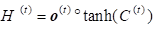
LSTM
were proposed as a solution to the vanishing gradients problem [12, 13]. On step![]() , there
is a hidden state and a cell state presented by vectors with length n.
The cell stores long-term information, and the LSTM can erase, write and read
information from the cell. The selection of which information is
erased/written/read is controlled by the following three dynamic gates with
length n: (a) forget gate (
, there
is a hidden state and a cell state presented by vectors with length n.
The cell stores long-term information, and the LSTM can erase, write and read
information from the cell. The selection of which information is
erased/written/read is controlled by the following three dynamic gates with
length n: (a) forget gate (![]() ) controls
what is kept vs forgotten, from previous cell state; (b) input gate (
) controls
what is kept vs forgotten, from previous cell state; (b) input gate (![]() ) controls what parts of the new
cell content are written to cell; (c) output gate (
) controls what parts of the new
cell content are written to cell; (c) output gate (![]() ) controls what parts of cell are output to
hidden state. On each time step, each element of the gates can be open (1),
closed (0), or somewhere in-between and their value is computed based on the
current context. New cell content (
) controls what parts of cell are output to
hidden state. On each time step, each element of the gates can be open (1),
closed (0), or somewhere in-between and their value is computed based on the
current context. New cell content (![]() ) determines
the new content to be written to the cell; cell state (
) determines
the new content to be written to the cell; cell state (![]() ) comes with two options: erase (“forget”)
some content from last cell state, and write (“input”) some new cell content; hidden
state (
) comes with two options: erase (“forget”)
some content from last cell state, and write (“input”) some new cell content; hidden
state (![]() ) reads (“output”) some content from the
cell (Figure1). Gates are applied using the Hadamard product. Equations (6)
represent the forward pass of LSTM [13].
) reads (“output”) some content from the
cell (Figure1). Gates are applied using the Hadamard product. Equations (6)
represent the forward pass of LSTM [13].
where ![]() ,
, ![]() ,
, ![]() and
and ![]() are respectively input vector to LSTM unit,
forget gate’s activation vector, input/update gate’s activation vector and
output gate’s activation vector;
are respectively input vector to LSTM unit,
forget gate’s activation vector, input/update gate’s activation vector and
output gate’s activation vector; ![]() ,
, ![]() and
and ![]() are in
turn hidden state vector, cell input activation vector and cell state vector.
are in
turn hidden state vector, cell input activation vector and cell state vector.
2.2. Hybrid Architecture: CNN Combined with LSTM
The combination of the CNN with the RNN-based LSTM allows to enmesh two architectures together where the CNN feeds features directly into the LSTM and the LSTM learns higher order sequential features. CNN is able to learn local response from temporal or spatial data but lacks the ability of learning sequential correlations while LSTM model uses these sequences of higher-level representations and further process them through its gates (Figure 1).
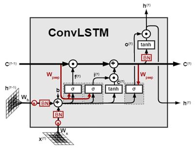
Using tensors allows further incorporation of CNN and LSTM for solving the forecasting of stock market. The data features are learned using convolution operations and the series of data over time are trained using LSTM what means the replacement of matrix multiplications in the input, forget and output gates of LSTM (6) with convolution operations denoted by * (7) [14].
Therefore, the state of a particular cell in the grid is determined by the input and past states of its neighbours’ states


where all inputs![]() , cell
outputs
, cell
outputs![]() , hidden states
, hidden states![]() , and
gates
, and
gates![]() ,
, ![]() and
and ![]() are 3-dimensional.
are 3-dimensional.
2.3 Attention-Based CNN – LSTM Topology
The classical time series prediction method ARIMA (auto regressive integrated moving average) cannot achieve satisfactory results for stock forecasting as it cannot define the data nonlinearity. The latter prevents mining of historical information of the stock market data in multiple periods of time [15].
Neural networks, however, have strong nonlinear generalization ability and their combination with ARIMA as a preprocessor improves the stock prediction results [16]. The pretrained Attention-based CNN-LSTM model based on sequence-to-sequence framework uses convolution to extract the deep features of the original stock data by convolution, and then LSTM network extracts the long-term series features [17, 18].
Additional fine tuning of hybrid model Attention-based CNN-LSTM with eXtreme Gradient Boosting improves efficiency of model as shown in [19, 20].
3. Performance Measures
Evaluating the performance of a prediction model is usually done by comparing the predicted values to the actual values what means by measuring the error between the two, where a lower error value indicates a better performance. The above approach named error-based evaluation metrics is commonly used in stock market prediction. It includes the mean absolute error, mean square error, root-mean-square deviation and R-squared error [2].
In our experiments, the performance of the stock market prediction models is measured by four indicators mean absolute error (MAE), mean square error (MSE), root mean square error (RMSE) and R-squared error (R2) where: a) MSE is a metric used to determine the average squared distance between the actual value and the predicted value; b) MAE calculates absolute errors, while MSE amplifies errors to their maximum by using the sum of squares of errors; c) RMSE is a commonly used metric for evaluating the accuracy of predictions by measuring the square root of the second sample moment of the differences between predicted and actual values. It is similar to MSE, with the only difference being the inclusion of the square root. It is therefore hard to determine which evaluation metric is more important; d) the coefficient of determination R2 is the proportion of the dependent variable that is predictable from the independent variable(s).
The mathematical expressions of the above error-based evaluation metrics are presented with equations (8, 9, 10, 11)
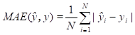
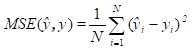
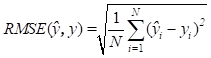
where![]() is the length of prediction,
is the length of prediction, ![]() and
and![]() represent
the predicted and measured (observed) value for the
represent
the predicted and measured (observed) value for the ![]() sample;
sample;
![]() is the average value. The value range for
R
2 is (0, 1). If
the values of MAE and RMSE are close to 0, then the error between the
respective predicted and real values is smaller and therefore the forecasting
accuracy is higher. The fitting degree of the model is better if the value of R2 is closer to 1.
is the average value. The value range for
R
2 is (0, 1). If
the values of MAE and RMSE are close to 0, then the error between the
respective predicted and real values is smaller and therefore the forecasting
accuracy is higher. The fitting degree of the model is better if the value of R2 is closer to 1.
4. Experiments
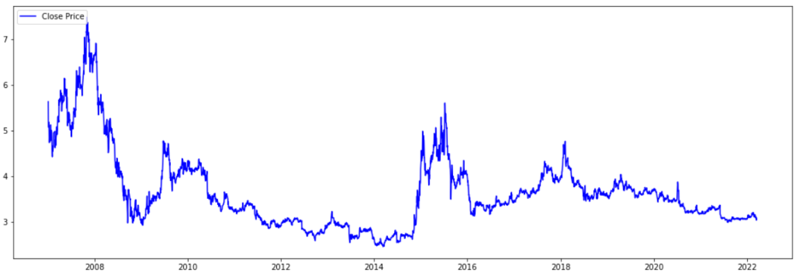
The experimental dataset used in this research is the stock market of China (601988.SH). It contains stock price data for the period of time January 1, 2007 to March 31, 2022 and is publicly available [21, 22]. It is shown in Figure 2. It has 20 columns having daily information about parameters such as opening price, closing price, maximum price, minimum price, trading volume, turnover rate and amount where the data in one day denotes a point of the sequence. For the purposes of stock market forecasting we selected the following limited part of dataset columns: 'open', 'high', 'low', 'close', and 'amount'. For all experiments ModelCheckpoint is used to save the best model during the training. The lookback (n_past) value is selected for different models with Adam as an optimizer and number of training epochs is set to 50.
Applying the scaling process in financial datasets prevents the stock from predicting higher values in the future that are not in the dataset. Our experiments with implementation of StandardScaler and MinMaxScaler prove that the first one is preferable due to the high numbers in the amount column while the second one squeezes the numerical data in the columns into a particular range. MinMaxScaler preferred by some researchers improves the machine learning model's accuracy but when applied to real problems it would affect the model generalization. The dataset is split randomly into training (all dataset except the last six months) and test (last six months).
The time-series forecasting models require setting the lookback value t as a parameter before the training. For example t = 20 means that model's instantaneous close price is predicted based on the previous 20 days in respective dataset columns.
4.1. Experimental Topologies and Performance
Our experiments for stock market prediction are organised in three experimental settings explained in this section.
In first experimental setting we propose three different hybrid topologies based on CNN_LSTM, Stacked_LSTM and GRU_BiLSTM where the lookback parameter takes respectively values 5, 10 and 20. The lookback values 5-10-20 are chosen because in the financial world, companies are expected to have significant changes in their stocks during the week (it is 5 because there are 5 weekdays in a week), 2 weeks (it is 10 because there are 10 weekdays in 2 weeks), and 1 month (it is 20 because there are 20 weekdays in a month). Performance evaluation of the above models is shown in Table 1.
Convolutional operation of CNN_LSTM model is designed as a tensor operation (n_samples, 1, 1, n_features, n_lookback) which differs from the usual CNN tensor operation (n_samples, n_lookback, n_features). Convolutional LSTM with 64 neurons in the first two layers is applied to the input dataset and second convolutional layer with 32 neurons is applied to its output. The extracted features are converted into a single long continuous linear vector by the flatten layer. The first layer of CNN Fully Connected Layer (FCL) is a dense layer with 16 neurons and the last one is a dense layer with 1 neuron (output).
Stacked_LSTM avoids overfitting while adjusting the depth of the model. In our experiments we include two hidden layers containing 64 neurons and 32 neurons because of trial and error. The model is built sequentially where the input shape is added into the first hidden layer containing the first 64 neurons with the feature offered by the TensorFlow library. Adding more than two LSTM layers to the topology might cause overfitting of the proposed neural architecture.
For many sequence labeling tasks it is beneficial to have access to both past (left) and future (right) contexts. However, the LSTM’s hidden state usually denoted by takes information only from the past, knowing nothing about the future. Effective solution to this problem is bi-directional LSTM (BiLSTM). The basic idea is to present each sequence forwards and backwards with two separate hidden states to capture past and future information, respectively. Then the two hidden states are merged to form the final output. Therefore, bi-directional LSTM is a sequence processing model that consists of two LSTMs: one taking the input in a forward direction, and the other in a backwards direction [19].
Table 1. Performance Evaluation of Stock-Prediction Models
|
Architecture |
MSE |
RMSE |
MAE |
R2 |
|
Conv_LSTM_5 |
0.0003 |
0.01742 |
0.0131 |
0.83128 |
|
Conv_LSTM_10 |
0.00029 |
0.01714 |
0.01271 |
0.8411 |
|
Conv_LSTM_20 |
0.00031 |
0.01766 |
0.01329 |
0.83851 |
|
Stacked_LSTM_5 |
0.00028 |
0,01670 |
0.01228 |
0.84492 |
|
Stacked_LSTM_10 |
0.00029 |
0.01693 |
0.0126 |
0.84498 |
|
Stacked_LSTM_20 |
0.00029 |
0.01697 |
0.01264 |
0.85094 |
|
GRU_BiLSTM_5 |
0.00028 |
0.01685 |
0.01289 |
0.84208 |
|
GRU_BiLSTM_10 |
0.00028 |
0.01676 |
0.01268 |
0.84799 |
|
GRU_BiLSTM_20 |
0.00036 |
0.01909 |
0.01462 |
0.81139 |
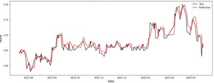
In the first group of experiments we also include the topology GRU-BiLSTM as it extracts historical hidden features more efficiently for some datasets [20]. Performance evaluation of the topologies included into the first experimental set is shown in Table 1, where Figure 3 determines that the Stack_LSTM_20 model has the highest accuracy (R2) of 0.85094 among the rest of the models used in the first experimental setting but it is lower than 0.88342 reported in [23]. GRU_BiLSTM model has the lowest performance with R2 score of 0.81139 when the lookback value is set to 20 - Table 1. Figure 3 and Figure 4 show the graphics of prediction and true values during the training.

Second experimental setting: The classical time series prediction method ARIMA cannot define the data nonlinearity and therefore prevents mining of historical information of the stock forecasting. We propose hybrid learning model integrating the time series ARIMA with neural networks because of their strong nonlinear generalization ability. The designed model incorporates ARIMA, a pretrained hybrid model attention-based CNN_BiLSTM with lookback of 20, where fine tuning of parameters is done by using light gradient boosting machine (LGBM). The stock market dataset is first preprocessed through ARIMA partial code of which is provided.
The proposed model is based on sequence-to-sequence framework, where the attention-based CNN is the encoder, and the bi-directional LSTM is the decoder. The deep features of the dataset are extracted by convolution operations and respectively BiLSTM gets the long-term data series features. Light gradient boosting regressor performs fine tuning, while fully extracting the information of the stock market in multiple periods. The LightGBM algorithm utilizes two novel techniques called Gradient-Based One-Side Sampling (GOSS) and Exclusive Feature Bundling (EFB) which allow the algorithm to run faster while maintaining a high level of accuracy.
Table 2 presents the performance of stock market dataset of the proposed model Attn_CNN_BiLSTM_LGBM and ACNN_BiLGBM/XGBoost proposed in [20]. Figure 5 and Figure 6 demonstrate the experimental results for the ACNN_BiLGBM/XGBoost and introduced in this paper Attn_CNN_BiLSTM_LGBM architecture with lookback parameter t = 20.
Table 2. Performance evaluation of proposed Attn_CNN_BiLSTM_LGBM and ACNN_BiLGBM/XGBoost
|
Model |
MSE |
R2 score |
MAE |
RMSE |
|
Attn_CNN_BiLSTM_LGBM |
0.00011 |
0.93909 |
0.00789 |
0.0103 |
|
ACNN_BiLGBM/XGBoost |
0.0002 |
0.88342 |
0.01126 |
0.01424 |
Analysis of MSE values for both approaches in solving stock market prediction task shows a decrease of almost 50% when using the new proposed model. Similarly, the R2 value, which indicates the pattern of the regression values, is much higher for the proposed architecture.
The green dashed line (Figure 5 and Figure 6) indicates that for model ACNN_BiLGBM/XGBoost the prediction value is at a peak position well above the actual value while for Attn_CNN_BiLSTM_LGBM this peak is at almost the same as the peak of the actual stock price. The red dashed line indicates that while the prediction values are far from the actual values in Figure 5, they are much closer to the actual values in Figure 6. The purple dashed line, on the other hand, predicts below the actual value in the graph for model ACNN_BiLGBM/XGBoost, while in the graph of Attn_CNN_BiLSTM_LGBM it matches the actual value almost exactly.
Therefore, Attn_CNN_BiLSTM_LGBM predicts the trends of the stock more accurately when compared to the rest of our models suggested in First Experimental Setting of this paper as well as the one in [20].
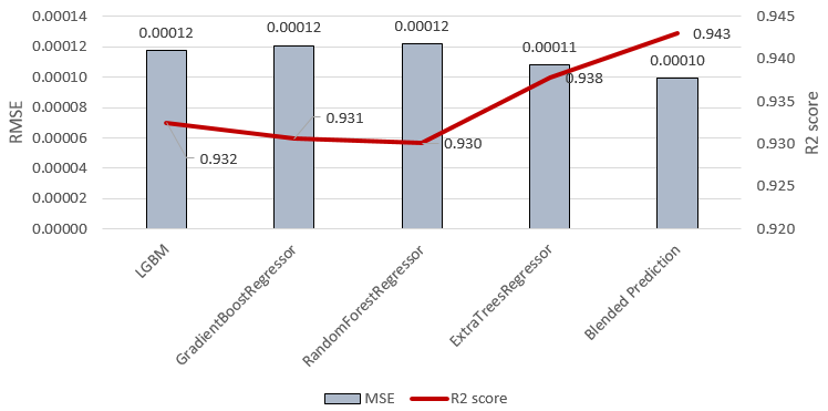
Table 3. Performance evaluation of ensemble model
|
Architecture |
MSE |
RMSE |
MAE |
R2 |
|
Attn_CNN_BiLSTM_LGBM |
0.000118 |
0.01034 |
0.00789 |
0.939091 |
|
Attn_CNN_BiLSTM_GBR |
0.000121 |
0.01099 |
0.00843 |
0.930596 |
|
Attn_CNN_BiLSTM_RFR |
0.000122 |
0.01103 |
0.00853 |
0.930076 |
|
Attn_CNN_BiLSTM_ETR |
0.000108 |
0.01041 |
0.00795 |
0.937702 |
|
Ensemble Model (EM) |
0.000099 |
0.00997 |
0.00757 |
0.94291 |
In third experimental setting we implement the light gradient boosting machine, gradient boosting regressor, random forest regressor (RFR), and extra-tree regressor (ET) with Attn_CNN_BiLSTM. In Table 3 we show the performance evaluation of these four architectures. It determines Attn_CNN_BiLSTM with random forest regressor as an architecture with the lowest performance and Attn_CNN_BiLSTM with light gradient boosting regressor as the one having the best evaluation results when compared to the other three experimental models.
The created ensemble prediction model combines the above four architectures and has the highest performance as shown in Table 3. EM implements weights average approach based on contribution of each ensemble member to the final EM performance. The EM prediction and true values are shown in Figure 7. Green, red, and purple arrows in this figure point to the areas which make a difference when compared to Attn_CNN_BiLSTM_RFR in Figure 8.
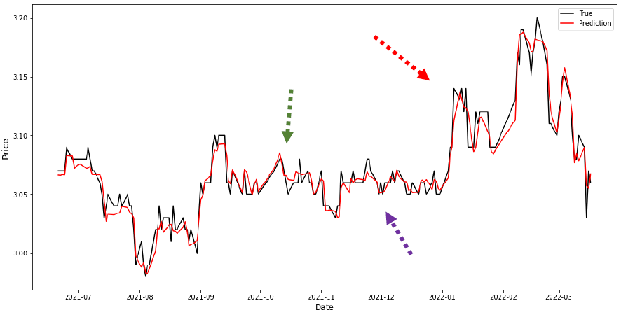
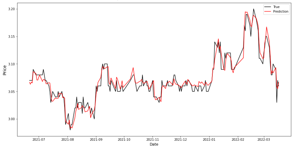
Figure 9 compares the R2 scores and RMSE values of Table 3 models. The line graph in red represents the R2 while the bar charts show the RMSE values of the models.
5. Conclusion
The stock market forecasting problems are mostly handled as time series task due to the specific time frame of the prediction which may range from minute level to day level. In this paper we propose several hybrid models which combine a deep learning approach by employing a convolutional LSTM, stack of LSTM and GRU_BiLSTM to study their effectiveness and applicability on the historical China stock market dataset. Our experiments show that Stack_LSTM_20 model captures better the complexity of stock market data and improves the forecasting accuracy for the stock market dataset.
We also propose a new hybrid architecture Attn_CNN_BiLSTM_LGBM which better models long sequences and therefore is able to solve long-term dependency problems more efficiently and accurately. While the Attention provides modelling of dependencies regardless to their distance in the input or output sequences, Attn_CNN additionally captures both local and global hidden patterns as well. Bi_LSTM provides the necessary flexibility and robustness in interpreting hidden patterns and their relations in complex datasets such as stock market while LGBM regressor does fine-tuning, allowing full mining of information in multiple periods. The experimental results prove that the proposed Attn_CNN_BiLSTM_LGBM achieves better performance in predicting the stock market than the one reported by other researchers.
Our ensemble model based on Attn_CNN_BiLSTM_ LGBM, Attn_CNN_BiLSTM and three more regressors implementing weighted average approach demonstrates the best performance when compared to the hybrid topologies suggested in this paper.
Future studies might be concentrated on improving generalization ability of deep learning models for stock market prediction and possibilities to integrate them with online learning approaches.
References
[1] J. Zou, Q. Zhao, Y. Jiao, H. Cao, Y. Liu, Q. Yan, E. Abbasnejad, L. Liu and J. Shi, "Stock Market Prediction via Deep Learning Techniques. A Survey", 2023. arXiv: 2212.12717.
[2] M. Ballings, D. Van den Poel, N. Hespeels, and R. Gryp, "Evaluating multiple classifiers for stock price direction prediction" in Expert systems with Applications 42, 20 (2015), pp. 7046-7056. View Article
[3] Z. Guo, H. Wang, Q. Liu and J. Yang, "A Feature Fusion Based Forecasting Model for Financial Time Series", Plos One 9(6): 172-200. View Article
[4] A. Rupesh Kamble, " Short and long term stock trend prediction using decision tree", in International Conference on Intelligent Computing and Control Systems (ICICCS), IEEE, 2017, pp. 1371-1375. View Article
[5] F.X. Satriyo D Nugroho, T. Bharata Adji and S. Fauziati, "Decision support system for stock trading using multiple indicators decision tree", in First International Conference on Information Technology, Computer, and Electrical Engineering, IEEE, 2014, pp. 291-296. View Article
[6] S. Prasadas, S. Padhy, "Support Vector Machines for Prediction of Futures Prices in Indian Stock Market", in International Journal of Computer Applications, 2012, 41(3): pp. 22-26. View Article
[7] Y. Bengio, A. Courville, P. Vincent, "Representation Learning: A Review and New Perspectives", IEEE Transactions on Pattern Analysis and Machine Intelligence 35(8): 2013, pp. 1798-1828. View Article
[8] J. Weiwei, "Applications of Deep Learning in Stock Market Prediction: Recent Report", Expert Systems 184 (2021), 115537. https://arxiv.org/pdf/2003.01859.pdf. View Article
[9] C. Szeged, W. Liu, Y. Jia, P. Sermanet, S. Reed, D. Anguelov, D. Erhan, V. Vanhoucke and A. Rabinovich, "Going deeper with convolutions", in Proceeding of the IEEE conference on Computer Vision and Pattern Recognition, Boston, MA, 2015, pp. 1-9. View Article
[10] K. Cho, B. van Merrienboer, C. Gulcehre, D. Bahdanau, F. Bougares, H. Schwenk and Y. Bengio, "Learning Phrase Representations using RNN Encoder-Decoder for Statistical Machine Translation", 2014, arXiv: 1406.1078. View Article
[11] Y. Yu, X. Si, C. Hu, and J. Zhang, "A Review of Recurrent Neural Networks: LSTM Cells and Network Architectures," Neural Computing, vol. 31, no. 7, pp. 1235-1270, Jul. 2019, doi: 10.1162/NECO_A_01199. View Article
[12] S. Hochreiter and J. Schmidhuber, "Long short-term memory", in Neural computation", 9(8): 1997, pp.1735-1780. View Article
[13] C. Olah, "Understanding LSTM Networks", 2015. https://colah.github.io/posts/2015-08-Understanding-LSTMs/
[14] I. Valova, N. Gueorguieva and S. Smudidonga, " Short-Term Traffic Forecasting Using Deep Learning", in Proceedings of the 7th World Congress on Electrical Engineering and Computer Systems and Sciences (EECSS'21) Prague, Czech Republic, July, 2021. Avestia Publishing, Paper No. MVML 102 DOI: 10.11159/mvml21.102, pp. MVML 102-1 - 102-8. View Article
[15] G. Zhang, "Time series forecasting using a hybrid ARIMA and Neural Network Model," in Neurocomputing, vol. 50, pp. 159-175, 2003. View Article
[16] I. Sutskever, O. Vinyals, and Q. V. Le, "Sequence to sequence learning with neural networks," in NeurIPS, 2014.
[17] S. Wiseman and A. M. Rush, "Sequence-to-sequence learning as beam search optimization," in EMNLP, 2016. View Article
[18] A. Vaswani, N. Shazeer, N. Parmar, J. Uszkoreit, L. Jones, A. N. Gomez, L. Kaiser, and I. Polosukhin, "Attention is all you need," in Proceedings of the 31st International Conference on Neural Information Processing Systems, December 2017, pp. 6000-6010.
[19] X. Hu, T. Liu, X. Hao and C. Lin, "Attention-based Conv-LSTM and Bi-LSTM networks for large-scale traffic speed prediction", Journal of Supercomputing 78, 2022, pp. 12686-12709. https://doi.org/10.1007/s11227-022-04386-7. View Article
[20] Z. Shi, Y. Hu, G. Mo, and J. Wu, "Attention-based CNN -LSTM and XGBoost hybrid model for stock prediction," Apr. 2022, doi: 10.48550/ arxiv.2204.02623. View Article
[21] J. Chung, C. Gulcehre, and K. Cho, "Empirical Evaluation of Gated Recurrent Neural Networks on Sequence Modeling", 2014. (Online) View Article
[22] www.tushare.pro; https://github.com/ waditu/ tushare. View Article
[23] V. Polepally, N. S. N. Reddy, M. Sindhuja, N. Anjali, and K. J. Reddy, “A Deep Learning Approach for prediction of Stock Price Based on Neural Network Models: LSTM and GRU,” 12th International Conference in Computational Communications and Network Technology, ICCCNT 2021, doi: 10.1109/ ICCCNT 51525.2021.9579782. View Article