Volume 3 - Year 2022 - Pages 01-12
DOI: 10.11159/jmids.2022.001
Comparison and Evaluation of Data Composition and Deep Learning Models in Archival Handwritten Digit Classification
Nathan LeBlanc, Iren Valova
University of Massachusetts Dartmouth, Computer and Information Systems Department
285 Old Westport Rd., Dartmouth, MA 02747, USA
Nleblanc2, ivalova@umassd.edu
Abstract - Archival maritime logs are well-preserved treasure throve of climate-related data. The analysis of these documents is instrumental to understanding historical climate trends and future predictions. Transcribing such handwritten logs depends on handwritten letter/digit recognition, which is our aim. The shortcomings of OCR (Optical Character Recognition) are manifesting in frequent confusion of digits and letters when it comes to archival handwritten documents. In this extension of conference and thesis work, two such methods are put to the test – convolutional (CNN) and long-short term memory (LSTM) neural networks (NN). A compound model of convolutional NN followed by LSTM is also considered. While all models register high accuracy, it is observed that the compound model performs faster with accuracy above the lone CNN. We also analyse dataset composition and test for size and balance.
Keywords: deep learning, compound models, convolutional neural networks, long-short term memory.
© Copyright 2022 Authors - This is an Open Access article published under the Creative Commons Attribution License terms. Unrestricted use, distribution, and reproduction in any medium are permitted, provided the original work is properly cited.
Date Received:2022-08-31
Date Accepted: 2022-09-10
Date Published: 2022-09-15
1. Introduction
A BBC article published in 2021 renewed our interest in identifying archival handwritten characters and symbols for purposes of transcribing. The end goal of such work is to automate the process of digitizing maritime logbooks to furnish historical data on climate details. Archiving of logbooks as scanned documents is further complicated due to their age and fragility, and the utlization of OCR.
Currently the most utilized method for the computer to recognize handwritten characters, OCR exhibits shortcomings in inability to tell the difference between “1” versus “7”, or “6” versus “8”. Adding distortions, folds, and artifacts, the OCR struggle would become more pronounced [1]. Deep learning models, more specifically CNN, have shown significant promise on a versatile scale of image recognition problems, including handwritten recognition [2, 3]. Recently, there have been some reports of attaching LSTM [4] at the output of CNN to further improve the deep learning model capabilities. One of our goals is to test whether such coupling (we named it compound model) delivers in terms of better accuracy, and time for the correct identification of handwritten digits. It must be said that currently, the only known method of highly accurate transcription of archival handwritten documents is by hand. We are aiming to challenge this by comparing the performance of CNN and a compound model of CNN followed by LSTM. We also explore the composition and balance of existing datasets.
The work in [5] started this research where we account for the shortcomings of OCR and aim to improve efficiency and efficacy through high-level deep learning architectures [6]. While the archived logbooks contain handwritten characters as well as other symbols, this work focuses on the digits. The dataset details are presented in section 2 with the deep learning architectures elaborated in section 3. Experiments are results are detailed in section 4, followed by conclusions.
2. Data
The dataset is collected mainly from National Oceanic and Atmospheric Administration (NOAA) which contains openly available weather-related reports from multiple locations spanning over the past 200 years [7]. Over 50 documents from NOAA containing weather report information from Worcester Massachusetts between the years of 1862 and 1950 are used for analysis and testing. All reports contain handwritten numerical information only, allowing for diverse handwritten information spanning over almost 100 years of data. The dataset contains handwritten numbers from 0 to 9 from at least three different authors. A sample of the data can be seen in Fig.1a.
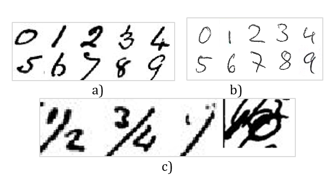
In addition to the digits, the NOAA archives contain a mix of special characters (Fig.1b) that are not used in the final dataset for this work but are noted as many of them contain digits. In addition to fractions of numbers, and writing that runs into other lines and numbers, notable issues include fading or doubling over existing writing.
For the purposes of distribution and balancing in training and validation datasets, an open-source dataset is considered, containing only handwritten digits (Fig.1c). This dataset contains 15,200 number images from at least 12 different authors.
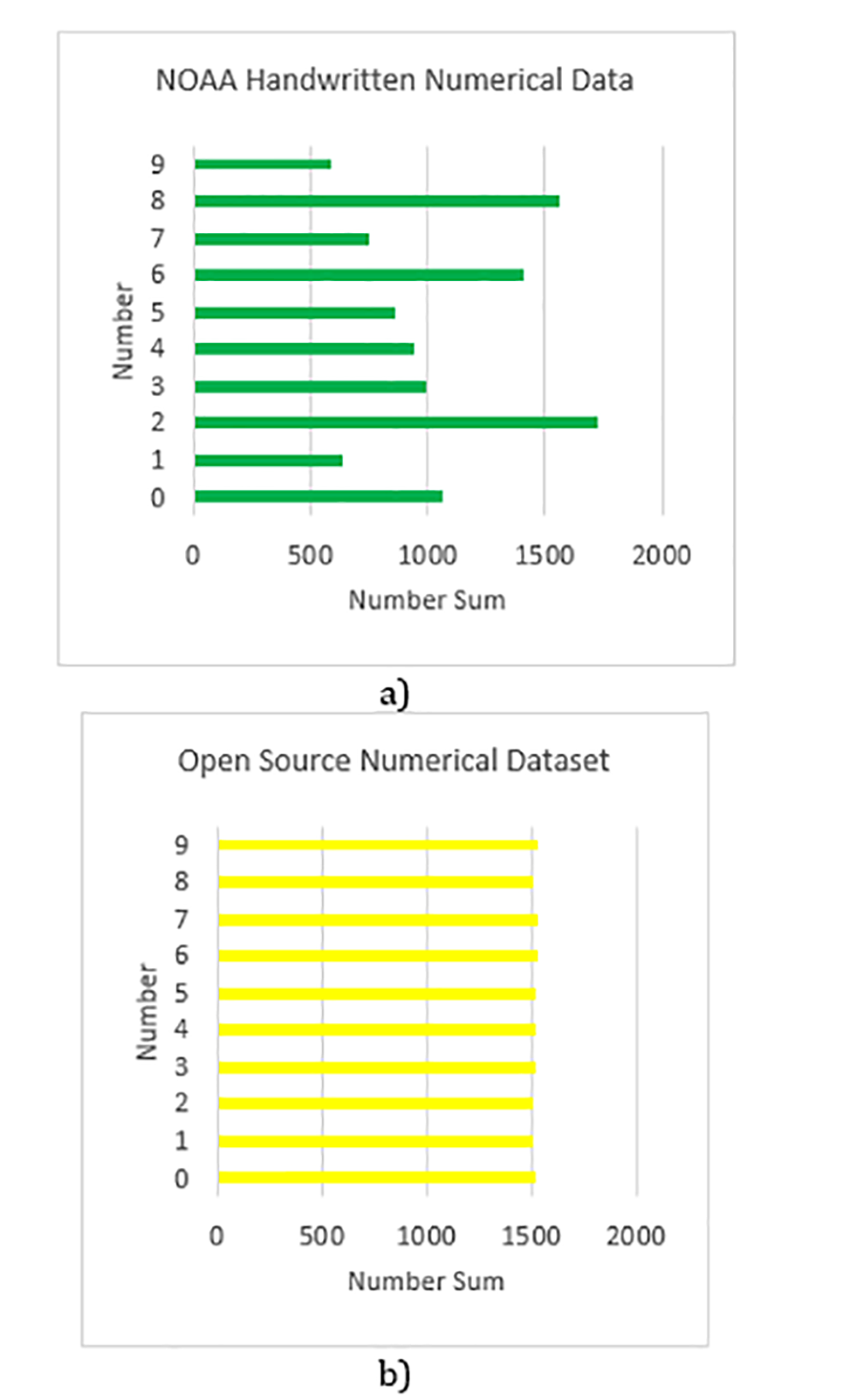
The NOAA dataset is distilled to 10,541 images of digits. Fig.2a illustrated the distribution of the various digits and conveys the heavy imbalance for some categories – only 537 images of “1”, but 1728 images of “2”.
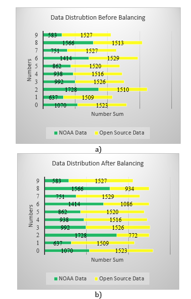
As is well-known [8], imbalance in datasets can lead to very poor performance. While augmenting is often the adopted resolution to this issue, here we have sourced additional 15,200 images of handwritten digits. Their distribution is illustrated in Fig.2b. Not all data from the open-source set is used to combat the imbalance. Only enough images are added to the NOAA dataset to ensure balanced representation of all digits, allowing for full “view” and consideration by the CNN and CNN+LSTM compound models. Post addition of images where needed most; each digit is represented by approximately 2,500 images. The distribution of NOAA/open-source datasets is shown in Fig.3a (augmentation without balance) and Fig.3b (after balance).
The final data used for testing and analysis contains 23,981 images of different numbers. These images come from the NOAA database and from open-source data. Combining the two datasets allows for greater diversification of training and exposure of the deep learning model to a larger variety of handwriting samples.
Considering the limited access to large dataset, we experiment with a small collection of digits (10,000). Details of this experiment are presented in section 4.
3. Deep Learning Models and Architectures
In this section we will briefly review the two main architectures utilized in our work – CNN and LSTM. While both are representatives of deep learning methods, i.e. operate on large to very large datasets, their methodology and aims are different with CNN focusing on image processing [9] and LSTM applicable to predictive analysis of time series data.
3. 1. Convolutional Neural Networks (CNN)
CNNs consist of two main portions (Fig.4a) – feature extraction to break down the image and emphasize key features; and classification to identify whether the image region of interest contains information of a particular group or class.
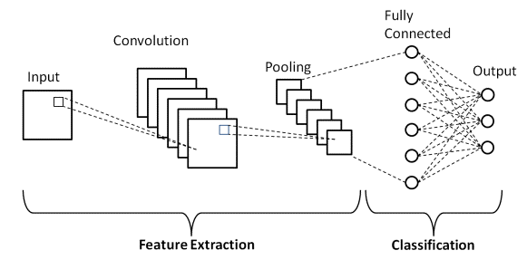
The four common layers of a CNN are: a convolutional layer, a pooling layer, fully connected layer, and a dropout layer. The convolutional layer extracts various features from the image. This is performed by sliding the filter over the image to centralize a matrix based on the pixel values for sections of the image. The dot product is then calculated between the values that exist in the image from the matrices created [10]. A pooling layer often follows a convolutional layer. It decreases the size of the feature map created from the convolutional layer, either by averaging or pulling the max values in the matrices. The fully connected layer is comprised of weighted connections between layers. This is where decisions on what the features represent are made [10]. The drop layer [11] removes some of the weighted connections between layers forcing the model to better generalize what feature make up data. The relationships among neurons are revised using optimizers. Thus, linearity is removed from the model allowing for accurate generalization [11].
3. 2. Long-Short Term Memory Neural Networks (LSTM)
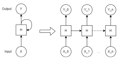
Recurrent neural networks (RNNs) contain a loop allowing for information to persist from one node to another as seen in Fig.5a. A loop from hidden state H to itself allows for the passing of information from one node in the network to the next [12]. RNNs are used in speech recognition, translation, and image captioning. If we want an RNN to predict the next word in a sentence, the sentence must remain short to allow for accurate results. The longer the sentence is, the worse the prediction will become as the model will struggle to link a correct output to an input that happens a long time before [13].
a)
b)
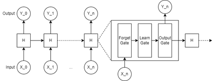
Long short-term memory networks are a special kind of RNN capable of learning long-term information. LSTMs contain a more complex structure in their hidden states than general RNNs (Fig.5b). An LSTM contains three main gates; a forget gate, a learn gate, and an output gate [12]. The forget gate uses a sigmoidal function to gauge information from 0 to 1 for what information should be kept, and what information should be forgotten. Once the forget gate has determined what information is useful, this information is passed to the learn gate. The learn gate determines what values need to be updated based on the information that was deemed useful from the forget gate. Once values are updated, they are received by the output gate. The output gate determines what the node is going to pass onto next node and what is going to output itself [14]. This process is repeated as many times as needed over the length of the data.
3. 3. Compound Model CNN+LSTM
The basic idea of CNN is image element(s) identification and classification. The core idea of LSTM is processing sequential data to memorize and make the connections leading to classifying the sequence gist. How are these two functionalities to be combined?
The CNN’s convolutions look at the image row by row, essentially “reading” it. With that, the pixels are transformed into sequences of features. Through additional layers, the most important features remain in the “sentence”. The LSTM then is responsible for making the connections between old and new information, determining what is to be learned or forgotten and to predict the probability of the “sentence” as one of the trained classes [15].
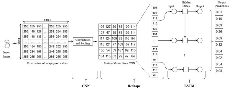
This process is simplified in Fig.6. An image is represented by grey scale pixel values. The image matrix of 64x64 serves as the CNN input for feature extraction and pooling. Once the feature extraction is complete, a new matrix with the final pooled values is reshaped into single columns of the values from the pooling matrix. The LSTM takes over these “sentences”. The final prediction is output as matrix with probabilities that the image belongs to a class from a list of given classes, in this case the classes are any number between 0 and 9. The class with the highest probability is predicted to be the number and the final prediction is outputted [16]. This process is done for all images in the dataset. We term the combination of feature extraction from a CNN and prediction from an LSTM as a compound network. This name embodies the ideas of composing two separate networks and putting them together to create a new network.

4. Experimentation and Results
For the purposes of training, validation, and testing, all images are converted to grey scale and sized as shown in Fig.7. Table 1 shows the distribution of the training, validation, and testing data per digit in the final utilized dataset. As a CNN, we utilize ResNet18 (Fig.8), which contains 18 layers [17]. There are 17 convolutional layers that feed into each other after performing convolution on the images. An average pooling layer is applied followed by a fully connected layer. Each convolutional layer in the Resnet architecture is followed by a batch normalization layer and a rectified linear activation function (ReLU) layer [18]. The compound model is illustrated in Fig.9.
Table 1: Large dataset distribution and content of training, validation, and testing subsets
|
Digit |
Total |
Train |
Test |
Validation |
|
Zero |
2593 |
1815 |
519 |
259 |
|
One |
2146 |
1502 |
429 |
215 |
|
Two |
2500 |
1750 |
500 |
250 |
|
Three |
2518 |
1763 |
503 |
252 |
|
Four |
2454 |
1202 |
490 |
245 |
|
Five |
2382 |
1668 |
476 |
238 |
|
Six |
2500 |
1750 |
500 |
250 |
|
Seven |
2278 |
1595 |
455 |
228 |
|
Eight |
2500 |
1750 |
500 |
250 |
|
Nine |
2110 |
1477 |
422 |
211 |
|
Totals |
23981 |
16787 |
4796 |
2398 |
4. 1. Small dataset – 10,000 images
Observing ResNet18 capability to learn through a smaller dataset shows promise in its ability to perform recognition.


a) CNN with small dataset
b) Compound model with small dataset
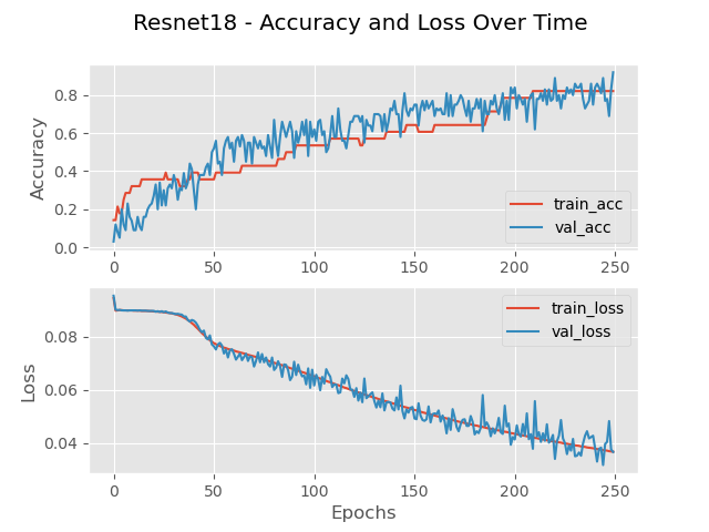
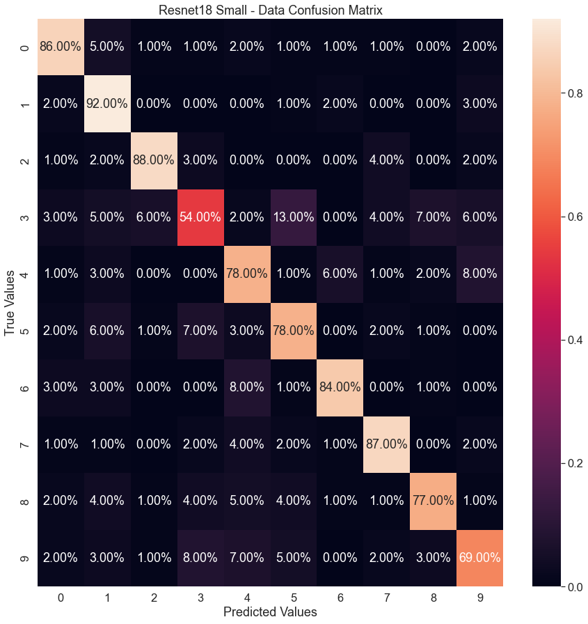
The dataset organization is the traditional 70/20/10 for training/validation/testing. The accuracy gradually increases only stopping once reaching the end of the run at 250 epochs (Fig.10a) with a minimum of 0.167 and a maximum of 0.82 for training. Similarly, the loss function continues to decrease only stopping due to run limitation. The final accuracy for this model on small dataset calculates at 79.3% accurate with a final loss of 0.037. The time to complete is 1,796.00 seconds (30 minutes). Ideally the loss should be small and the accuracy high, which is exactly what this model portrays. These progressions show that the model is learning accurately and correctly. Low loss indicates that the model is not missing details that exist in the images. A high accuracy indicates that the model is correctly predicting what number the image is supposed to represent. In the confusion matrix (Fig.11a), mistakes that the network makes become clear. A low accuracy in the recognition the number ‘3’ and ‘9’ attribute the low accuracy of the network. While the network still struggles across the board above 90% accuracy on the number ‘1’.
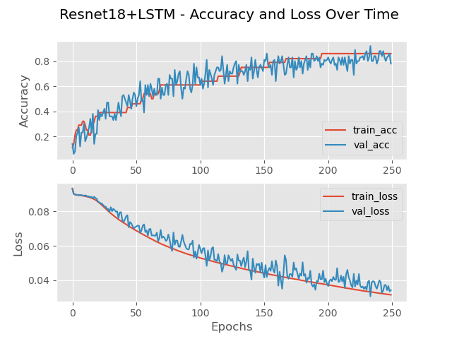
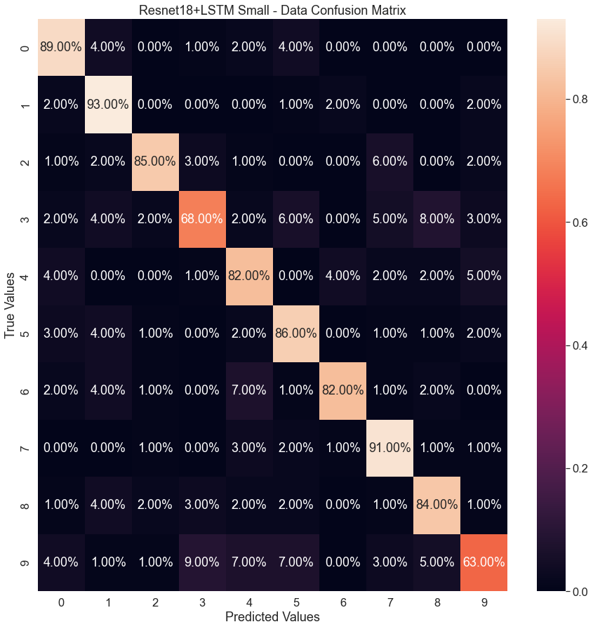
With the compound model presented in Fig.10b, accuracy and loss are very close to the ResNet registering minimum of 0.174 and a maximum of 0.88. The more noticeable difference is in the confusion matrix (Fg.11b). While the overall accuracy calculates at the same value ResNet-18 by itself, the classification of data appears more evenly distributed where no one number is misclassified versus the other numbers as well as avoiding the 54% accuracy for digit 3.
4. 2. Large dataset – 23981 images
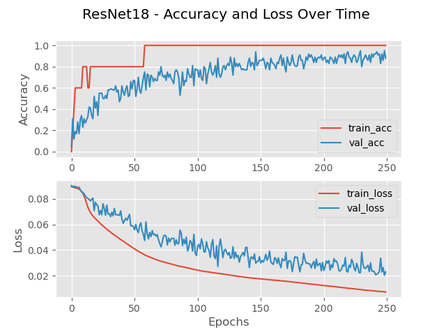
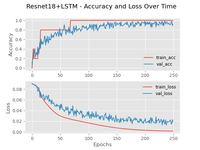
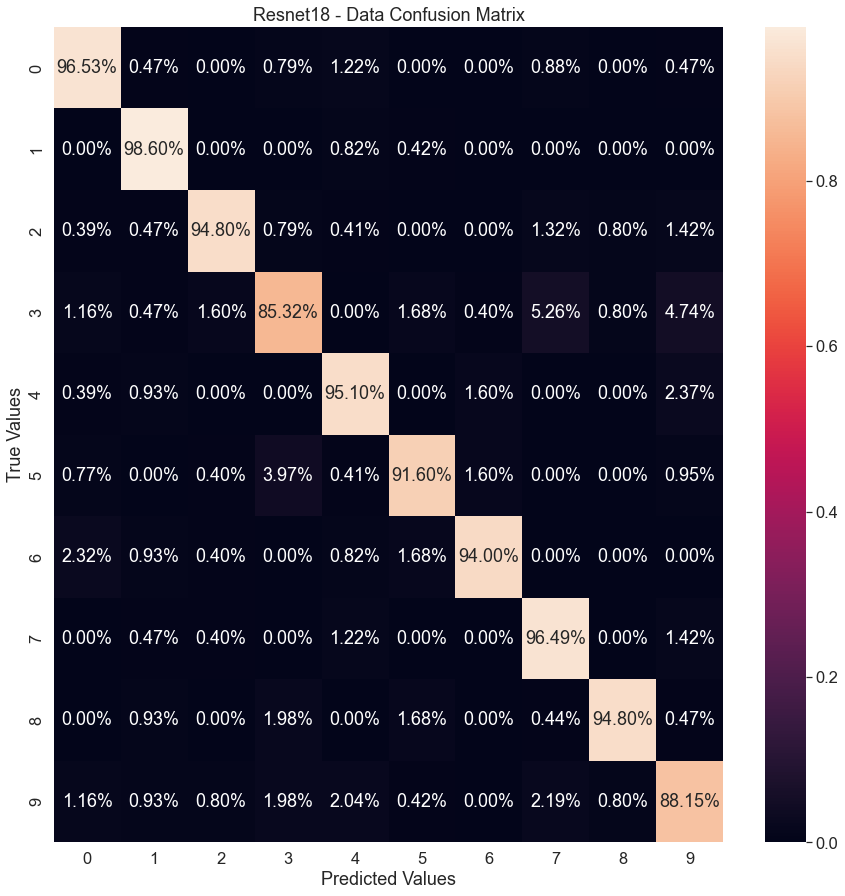
Over the course of the run time, which took 2,807.80 seconds (47 minutes), a gradual increase in validation accuracy and gradual decline in validation loss is seen. This validation accuracy can be seen to slowly increase to 93.5% over the course of the 250 epochs (Fig.12a). More dramatic is the training accuracy, spiking from 0.8 to 1 in around 20 epochs (starting minimum of 0.012). After the initial spike, the model slows down until it reaches a training accuracy of 1.0 at around 60 epochs. The final classification of digits can be seen in the confusion matrix (Fig.13a), showing that the model does not struggle in validating what data it was viewing. All number classifications scored over 85%, with eight out of ten classifications being over 90%.
a)
b)
a) CNN large dataset
b) Compound model large dataset
The compound model also uses ResNet-18 for consistency of experimentation. Instead of sending all information from the fully connected layer to a SoftMax layer for output, the data is reshaped via flattening for LSTM consumption. This decreases the number of channels from 3 to 2. Then a time distribution reshape follows, which assigns the data to be broken into segments like that of time series data (Fig.6). The LSTM must contain an input size equal to the reshape layers output. From the reshaping output the number of hidden layers can be decided, for this testing 32 hidden layers are determined as best (empirical and documented [14] evidence).
The final accuracy for CNN+LSTM compound model is 95.6% with a loss of 0.004 - Fig.12b – illustrating similar minimum and maximum as the CNN. The runtime is recorded at 2442.70 seconds (41 minutes). The compound model vastly outperforms the ability of a CNN on its own. The identification reaches testing accuracies (Fig.13b) between 99.5% and 91.9%. Compared with the CNN alone (Fig.13a), the compound model shows a significant improvement in performance.
In our experiments Adam optimizer is used with a learning rate of 0.000001. This optimizer allows for gradient descent with momentum learning, which implies sparing use of memory and training time [19]. Mean square error is used for the loss calculations. Training is completed in 250 epochs and batch training size is 64.
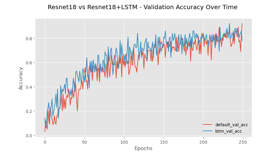
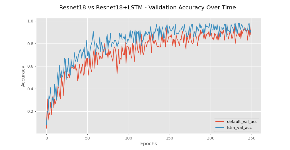
To better illustrate the gains of utilizing a compound model, Fig.14 presents the training and validation accuracies for the small and large datasets. In the small dataset experiment (Fig.14a), from the start of training to around 150 epochs, the compound model stays above the performance of the CNN. It is not until around 150 epochs that the models begin to have similar performance to each other with no noticeable difference. Figs.11b and 13b paint a better picture to understand the reason behind these results. Each of these figures shows the confusion matrix breakdown for the models. In Fig.9b the spread of predictions is far more prevalent than that of Fig.10b. This conciseness comes with the addition of the LSTM. Under testing more data further evidence is found further validating the quality of adding an LSTM to a CNN network.
The large dataset (Fig.14b) shows an even clearer difference between the lone CNN and the compound model. There is a clear contrast in ability of the compound model over just the CNN. Despite each network getting over a 90% accuracy, the process of reaching that accuracy in better performed by the compound network. From begin to end, the compound network stays above the lone CNN in ability to accurately identify the data. The minimum/maximum accuracy range is as follows: Fig.14a – 0.03 – 0.97 (CNN) and 0.17 – 0.98 (compound model); Fig.14b – 0.03 – 0.97 (CNN) and 0.17 – 0.98 (compound model). The further feeds the idea that the compound network outperforms the CNN in accuracy. To view these types of results more data must be added to the network. Seemly the more data, the better the performance compound model as has been seen with base CNN models [8].
a)

b)
a)
b)
4. 3. Results discussion
To fully understand the ability of adding an LSTM to a CNN an observation of time must be made. In Table 2 a complete breakdown of run times can be seen. Notably the more data that is run through the models, the longer the model takes to complete a full analysis. However, Table 2 clearly show the advantage of the compound model. Obviously, models with an LSTM train faster than those without. This leads to the belief that compounding decreases training time, reduces time needed to adjust any parameter leading to faster runs when training. All the models start slow and then speedup as their parameters adjust. Since the compound models are adjusting more accurately and faster than just a CNN, the runtime appears to go down in later runs. This information further supports that compound model (CNN+LSTM) mostly outperforms a CNN when dealing with handwritten data.
Table 2: Runtime of models
|
Model |
Runtime |
|
CNN – Small Dataset |
1,946.94 sec (32.45 min) |
|
Compound – Small Dataset |
1,227.41 sec (20.46 min) |
|
CNN – Large Dataset |
2,807.80 sec (46.80 min) |
|
Compound – Large Dataset |
2,4442.70 sec (40.70 min) |
Table 3: Misclassified Images for Resnet18
|
Image |
True |
Prediction |
Notes |
 |
8 |
7 |
General Misclassification |
 |
5 |
3 |
Missing defining features |
 |
3 |
6 |
Fading, Missing defining features |
 |
3 |
9 |
Poor crop on resizing of image |
 |
9 |
1 |
Poor shape where 9 in malformed |
Table 4: Misclassified Images for Resnet18+LSTM
|
Image |
True |
Prediction |
Notes |
 |
3 |
9 |
Poor shape where 3 has extra features |
 |
8 |
3 |
General Misclassification |
 |
4 |
6 |
Poor shape - 4 appears as 6 |
 |
9 |
4 |
Poor shape - 9 is malformed |
 |
0 |
6 |
Poor shape - 8 is malformed |
As with any learning system, there are mishaps. To further understand the failings of the models, both with and without an LSTM, further observation is made only on images that are misidentified. Table 3 illustrates the common CNN misclassifications. We conjecture the most common causes to be fading in portions of the image, cropping causing features to be removed, and odd shapes and writings of the numbers. The worst performing numbers for classification are still ‘3’ and ‘9’ in the compound model.
Table 4 shows a breakdown of the most common reasons for misclassification across the dataset. Noticeably the most common reason for the images to be misclassified is due to strange shapes of the images when written. While some misidentifications are due to general failure, most happen due to creative styles of writing. Understanding of the reasons behind deep learning models’ misclassification allows for deeper appreciation of the necessity of big datasets. While 23,981 seems like a considerable number capturing generalization of numbers for all types of styles of writing can be problematic.
5. Conclusion
In conclusion, we are exploring deep learning models for the purposes of archival handwritten document digitization. Such operation implies recognizing the characters and symbols and transcribing the archival logbooks in electronic format. While OCR has been a good standard for many years, its deficiencies in handwritten documents are well documented. We explore the deep learning model of CNN, but, more importantly, introduce a compound model of CNN and LSTM to handle the task mode efficiently (in less time) and more efficaciously (higher accuracy). The presented proof-of-concept work is limited to handwritten digits sourced from NOAA archives [20]. The results lead us to conclude that CNN (ResNet-18 in our case) is efficient registering accuracies spanning 88% (for “9”) to 98.6% (for “1”). The training process clocked at 47 minutes.
Additionally, the compound model consisting of CNN + LSTM (Resnet18 with some modifications at the end to accommodate the LSTM input needs) is very efficient at accuracies of 91.94% (“9”) to 99.3% (“1”). The training process is shorter at 41 minutes.
While we are working with augmented NOAA and open-source dataset of 23,981 images, to alleviate further some misclassifications, larger dataset is needed with more diverse samples.
We have also confirmed the need for large and balanced datasets for the successful training of deep learning models. In addition, the run times of the compound model are promising in their adoption for purposes of archival handwritten digits.
In summary, it is evident that compound models are better than their individual parts. More work is needed to accurately understand the handwriting of archival documents, and the automation in the translation of old texts.
References
[1] H. Schantz, The History of OCR, Optical Character Recognition. Recognition Technologies Users Association. 1982.
[2] S. Ahlawat, A. Choudhary, A. Nayyar, S. Singh, and B. Yoon “Improved Handwritten Digit Recognition Using Convolutional Neural Networks (CNN).” Sensors. 2020; 20(12):3344. View Article
[3] H. Pham, A. Setlur, S. Dingliwal, T.H. Lin, B. Poczos, K. Huang, Z. Li, J. Lim, C. McCormack, and T. Vu, “Robust Handwriting Recognition with Limited and Noisy Data,” 2020 17th International Conference on Frontiers in Handwriting Recognition (ICFHR), 2020, pp. 301-306, doi: 10.1109/ICFHR2020.2020.00062. View Article
[4] K. Dutta, P. Krishnan, M. Mathew, and C. V. Jawahar, “Improving CNN-RNN Hybrid Networks for Handwriting Recognition,” 2018 16th International Conference on Frontiers in Handwriting Recognition (ICFHR), 2018, pp. 80-85. View Article
[5] M. McGrath, “Climate Change: IPCC Report is ‘Code Red for Humanity’” BBC News. August 2021. [Online]. Available View Article
[6] S. Xu, Q. Wu, S. Zhang, Application of Neural Network in Handwriting Recognition. Stanford University. 2020.
[7] NOAA Database. “Climate Data Records (CDR).” National Centre for Environmental Information. 2022. [Online]. Available View Article
[8] I.Valova, C. Harris, T. Mai, and N. Gueorguieva, “Optimization of Convolutional Neural Networks for Imbalanced Set Classification”, 24th Intl Conf. Knowledge-Based and Intelligent Information & Engineering Systems, Procedia Computer Science 176 (2020) 660–669 View Article
[9] S. Balaji, “Binary Image classifier CNN using TensorFlow.” Medium. Aug 28, 2020. [Online]. Available View Article
[10] A. Geron, Hands-on Machine Learning with Scikit-Learn, Keras, and Tensorflow. O’Reilly Media. 2019.
[11] H. Wu, and G. Xiaodong. “Towards dropout training for convolutional neural networks.” Neural Networks, Vol. 71, 2015. 0893-6080. View Article
[12] A. Sherstinsky, “Fundamentals of Recurrent Neural Network (RNN) and Long Short-Term Memory (LSTM) network.” Physica D: Nonlinear Phenomena, Vol. 404, 2020. View Article
[13] N. Manaswi, RNN and LSTM. In: Deep Learning with Applications Using Python. Apress, Berkeley, CA. 2018. View Article
[14] S. Zhang, Y. Wu, T. Che, Z. Lin, R. Memisevic, R. Salakhutdinov, and Y. Bengio, "Architectural complexity measures of recurrent neural networks." Advances in Neural Information Processing Systems 29. 2016.
[15] W. Jiang, Y. Yang, J. Mao, Z. Huang, C. Huang, W. Xu, “CNN-RNN: A Unified Framework for Multi-Label Image Classification.” Proceedings of the IEEE Conference on Computer Vision and Pattern Recognition (CVPR), 2016, pp. 2285-2294. View Article
[16] A. Graves, S. Fernandez, F. Gomez, and J. Schmidhuber “Connectionist Temporal Classification: Labelling Unsegmented Sequence Data with Recurrent Neural Networks.” Association for Computing Machinery. 2006. View Article
[17] R. Farheen, M. Usman, and C. Khan, “Original ResNet-18 Architecture.” ResearchGate. 2019. [Online]. Available View Article
[18] A. Kandpal, “Residual Neural Network.” Open Genus. 2022. View Article
[19] D. Kingma and J. Ba. “Adam: A Method for Stochastic Optimization.” ArXiv preprint ArXiv:1412.6980. 2014. View Article
[20] N. LeBlanc, “Improving Handwritten Text Identification Through Convolutional and Recurrent Neural Networks”, MS Thesis, University of Massachusetts Dartmouth Library Archive, 2022.

